Discontinuous Galerkin Methods
for Conservation Laws

The Finite Volume Method = Galerkin FEM

• Consider the 1-D conservation law \[\begin{aligned} \frac{\partial u}{\partial t} + \frac{\partial f(u)}{\partial x} = 0 \end{aligned}\]

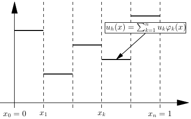
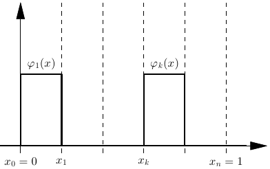
• Look for solutions in space of piecewise constant functions \(V_h\) \[\begin{aligned} u_h(x) = \sum_{k=1}^n u_k \varphi_k(x),\qquad \varphi_k(x) = \left\{ \begin{array}{rl} 1 & x_{k-1}<x<x_k \\ 0 & \text{otherwise} \end{array} \right. \end{aligned}\]

The Finite Volume Method = Galerkin FEM

• Galerkin formulation: Find \(u_h\in V_h\) such that \[\begin{aligned} \int_0^1 \frac{\partial u_h}{\partial t} v\,dx +\int_0^1 \frac{\partial f(u_h)}{\partial x} v\,dx = 0,\quad \forall v\in V_h \end{aligned}\]

• Set \(v=\varphi_k= \begin{cases} 1 & x\in[x_{k-1},x_k] \\ 0 & \text{otherwise} \end{cases}\) \[\begin{aligned} \hspace{-1.6cm} \int_{x_{k-1}}^{x_k} \frac{\partial u_h}{\partial t}\,dx +\int_{x_{k-1}}^{x_k} \frac{\partial f(u_h)}{\partial x}\,dx = 0 \Longleftrightarrow \int_{x_{k-1}}^{x_k} \frac{\partial u_h}{\partial t}\,dx +\left[ f(u_h(x))\right]_{x_{k-1}}^{x_k} = 0 \end{aligned}\]

• Since \(u_h\) is discontinuous at \(x_k\) and \(x_{k-1}\), use a numerical flux function \(F(u_R,u_L)\) to obtain: \[\begin{aligned} h\frac{\partial u_k}{\partial t} + F(u_{k+1},u_{k}) - F(u_k,u_{k-1}) = 0 \end{aligned}\]

• This is a standard finite volume method on a uniform grid

The Discontinuous Galerkin Method

• Generalize the Galerkin FEM approach to the space of piecewise polynomials of degree \(p\)

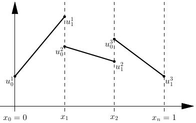
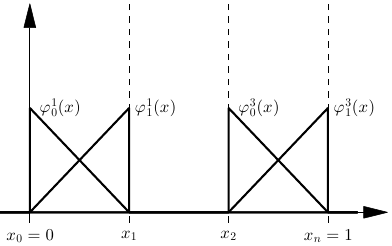
• Nodal representation with values \(u_i^k\) for local node \(i\) in element \(k\): \[\begin{aligned} u_h(x) = \sum_{k=1}^n \sum_{i=0}^p u_i^k \varphi_i^k(x) \end{aligned}\]

• Example, piecewise linear functions (\(p=1\)):

The Discontinuous Galerkin Method

• Galerkin formulation: Find \(u_h\in V_h\) such that \[\begin{aligned} \int_0^1 \frac{\partial u_h}{\partial t}v\, dx + \int_0^1 \frac{\partial f(u_h)}{\partial x}v\,dx = 0,\quad \forall v\in V_h \end{aligned}\]

• Set \(v=\varphi_i^k\) and integrate by parts \[\begin{aligned} \hspace{-10mm} \int_{x_{k-1}}^{x_k} \frac{\partial u_h}{\partial t} \varphi_i^k\,dx + \left[ f(u_h(x))\varphi_i^k(x) \right]_{x_{k-1}}^{x_k} -\int_{x_{k-1}}^{x_k} f(u_h(x))\frac{d\varphi_i^k}{dx}\,dx = 0 \end{aligned}\]

• Use a numerical flux function \(F(u_R,u_L)\) at the discontinuities \[\begin{aligned} &\int_{x_{k-1}}^{x_k} \frac{\partial u_h}{\partial t} \varphi_i^k\,dx + F(u_0^{k+1},u_p^k)\varphi_i^k(x_{k}) - F(u_0^k,u_p^{k-1})\varphi_i^k(x_{k-1}) \\ &-\int_{x_{k-1}}^{x_k} f(u_h(x))\frac{d\varphi_i^k}{dx}\,dx = 0 \end{aligned}\]

The Discontinuous Galerkin Method

• Example: \(f(u)=u\), \(F(u_R,u_L)=u_L\) \[\begin{aligned} &\hspace{-1.2cm}\int_{x_{k-1}}^{x_k} \frac{\partial}{\partial t} \left( \sum_{j=0}^p u_j^k \varphi_j^k(x) \right) \varphi_i^k\,dx - \int_{x_{k-1}}^{x_k} \left( \sum_{j=0}^p u_j^k \varphi_j^k(x) \right) \frac{d\varphi_i^k}{dx}\,dx \\ & +u_p^k\varphi_i^k(x_k)-u_p^{k-1}\varphi_i^k(x_{k-1}) = 0 \end{aligned}\]

• Rearrange to obtain a linear system of equations \[\begin{aligned} M^k \dot{\boldsymbol{u}}^k-C^k\boldsymbol{u}^k + \begin{pmatrix} -u_p^{k-1} \\ 0 \\ \vdots \\ 0 \\ u_p^k \end{pmatrix} = 0 \end{aligned}\] for element \(k\), with elementary matrices \[\begin{aligned} M_{ij}^k = \int_{x_{k-1}}^{x_k} \varphi_i^k\varphi_j^k\,dx\text{ and } C_{ij}^k = \int_{x_{k-1}}^{x_k} \frac{d\varphi_i^k}{dx}\varphi_j^k\,dx \end{aligned}\]

Calculating Elementary Matrices

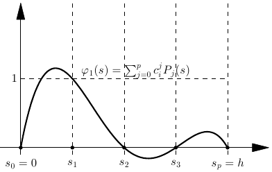
• Consider an element of degree \(p\), width \(h\), and a nodal basis for the points \(s_i\), \(i=0,\ldots,p\)

  • Equidistant points \(s_i=ih/p\) only good for low \(p\)

  • Better choice: Chebyshev or Gauss-Lobatto nodes

• Write basis functions as \(\varphi_i(s) = \sum_{j=0}^p c_i^j P_j(s)\), where \(P_j\) is a basis for the polynomials of degree \(p\)

  • Monomial basis \(P_j(s) = s^j\) only good for low \(p\)

  • Better choice: Orthogonal polynomials, e.g. Legendre

• Nodal basis functions are defined by \[\begin{aligned} \varphi_i(s_j) = \delta_{ij} = \begin{cases} 1 & i=j \\ 0 & i\ne j \end{cases} \end{aligned}\]

• Produces a linear system of equations

Calculating Elementary Matrices

• The linear system of equations has the form \[\begin{aligned} \hspace{-12mm} \begin{pmatrix} P_0(s_0) & P_1(s_0) & \cdots & P_p(s_0) \\ P_0(s_1) & P_1(s_1) & \cdots & P_p(s_1) \\ \vdots & \vdots & \ddots & \vdots \\ P_0(s_p) & P_1(s_p) & \cdots & P_p(s_p) \\ \end{pmatrix} \begin{pmatrix} c_0^0 & c_1^0 & \cdots & c_p^0 \\ c_0^1 & c_1^1 & \cdots & c_p^1 \\ \vdots & \vdots & \ddots & \vdots \\ c_0^p & c_1^p & \cdots & c_p^p \\ \end{pmatrix} = \begin{pmatrix} 1 & & & \\ & 1 & & \\ & & \ddots & \\ & & & 1 \end{pmatrix} \end{aligned}\] or \(VC=I\), which gives the coefficient matrix \(C=V^{-1}\)

• Use Gaussian quadrature or explicit polynomial integration to compute the elementary matrices \[\begin{aligned} M_{ij}&=\int_0^h \varphi_i(s)\varphi_j(s)\, ds \\ C_{ij}&=\int_0^h \varphi_i'(s)\varphi_j(s)\, ds \end{aligned}\]

The DG method – General systems of conservation laws

• (Reed/Hill 1973, Lesaint/Raviart 1974, Cockburn/Shu 1989-)

• Consider a first-order system of conservation laws: \[\begin{aligned} \boldsymbol{u}_t + \nabla \cdot \boldsymbol{F}(\boldsymbol{u}) = 0 \end{aligned}\]

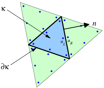
• Triangulate domain \(\Omega\) into elements \(\kappa\in \mathcal{T}_h\)

• Seek approximate solution \(\boldsymbol{u}_h\) in space of element-wise polynomials: \[\begin{aligned} \boldsymbol{V}_h^p = \{\boldsymbol{v}\in L^2(\Omega) : \boldsymbol{v}|_\kappa\in P^p(\kappa) \,\,\forall \kappa \in T_h \} \end{aligned}\]

• Multiply by test function \(\boldsymbol{v}_h\in\boldsymbol{V}_h^p\), integrate over element \(\kappa\): \[\begin{aligned} \int_\kappa \left[ (\boldsymbol{u}_h)_t + \nabla \cdot \boldsymbol{F}(\boldsymbol{u}_h) \right] \boldsymbol{v}_h\, d\boldsymbol{x} = 0 \end{aligned}\]

The DG method – General systems of conservation laws

• Integrate by parts: \[\begin{aligned} \hspace{-5mm} \int_\kappa \left[(\boldsymbol{u}_h)_t\right] \boldsymbol{v}_h\,d\boldsymbol{x} - \int_\kappa \boldsymbol{F}(\boldsymbol{u}_h) \nabla\boldsymbol{v}_h\,d\boldsymbol{x} + \int_{\partial\kappa} \hat{\boldsymbol{F}}(\boldsymbol{u}_h^+,\boldsymbol{u}_h^-,\hat{\boldsymbol{n}}) \boldsymbol{v}_h^+\,ds = 0 \end{aligned}\] with numerical flux function \(\hat{\boldsymbol{F}}(\boldsymbol{u}_L,\boldsymbol{u}_R,\hat{\boldsymbol{n}})\) for left/right states \(\boldsymbol{u}_L\),\(\boldsymbol{u}_R\) in direction \(\hat{\boldsymbol{n}}\) (Godunov, Roe, Osher, Van Leer, Lax-Friedrichs, etc)

• Global problem: Find \(\boldsymbol{u}_h\in\boldsymbol{V}_h^p\) such that this weighted residual is zero for all \(\boldsymbol{v}_h\in\boldsymbol{V}_h^p\)

• Error \(= \mathcal{O}(h^{p+1})\) for smooth solutions  
   
   
  

The DG Method – Observations

• Reduces to the finite volume method for \(p=0\): \[\begin{aligned} (\boldsymbol{u}_h)_t A_\kappa + \int_{\partial\kappa} \hat{\boldsymbol{F}}(\boldsymbol{u}_h^+, \boldsymbol{u}_h^-,\hat{\boldsymbol{n}})\,ds = 0 \end{aligned}\]

• Boundary conditions enforced naturally for any degree \(p\)

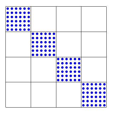
• Block-diagonal mass matrix (no overlap between basis functions)

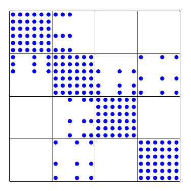
• Block-wise compact stencil – neighboring elements connected

Convection-Diffusion, the LDG method

• Consider the convection-diffusion equation \[\begin{aligned} \frac{\partial u}{\partial t} + \frac{\partial f(u)}{\partial x} - \mu\frac{\partial ^2u}{\partial x^2} = 0 \end{aligned}\]

• Split into system of first order equations: \[\begin{aligned} \frac{\partial u}{\partial t} + \frac{\partial f(u)}{\partial x} - \mu\frac{\partial \sigma}{\partial x} &= 0 \\ \frac{\partial u}{\partial x} &= \sigma \end{aligned}\]

• Galerkin formulation: Find \(u_h,\sigma_h \in V_h\) such that \[\begin{aligned} &\int_0^1 \frac{\partial u_h}{\partial t}v\, dx + \int_0^1 \left(\frac{\partial f(u_h)}{\partial x} - \mu\frac{\partial \sigma_h}{\partial x} \right) v\,dx = 0,\quad \forall v\in V_h \\ &\int_0^1 \frac{\partial u_h}{\partial x}\tau\,dx = \int_0^1 \sigma_h \tau\,dx,\quad \forall \tau\in V_h \end{aligned}\]

Convection-Diffusion, the LDG method

• Set \(v,\tau=\varphi_i^k\) and integrate by parts \[\begin{aligned} \hspace{-10mm} &\int_{x_{k-1}}^{x_k} \frac{\partial u_h}{\partial t} \varphi_i^k\,dx + \left[ \left(f(u_h(x)) - \mu\sigma_h(x)\right)\varphi_i^k(x) \right]_{x_{k-1}}^{x_k} \\ & \qquad\qquad-\int_{x_{k-1}}^{x_k} \left(f(u_h(x))-\mu\sigma_h(x) \right)\frac{d\varphi_i^k}{dx}\,dx = 0, \qquad \forall i,k\\ &\left[ u_h(x)\varphi_i^k(x) \right]_{x_{k-1}}^{x_k} \\ & \qquad\qquad -\int_{x_{k-1}}^{x_k} u_h(x) \frac{d\varphi_i^k}{dx}\,dx = \int_{x_{k-1}}^{x_k} \sigma_h(x) \varphi_i^k \,dx,\qquad \forall i,k \end{aligned}\]

• Use numerical flux functions \(\hat{f}(u_R,u_L)\), \(\hat{\sigma}(\sigma_R,\sigma_L)\), \(\hat{u}(u_R,u_L)\) at the discontinuities

• Example: \(f(u)=u\), \(\hat{f}(u_R,u_L) = u_L\), \(\hat{\sigma}(\sigma_R,\sigma_L) = \sigma_L\), \(\hat{u}(u_R,u_L) = u_R\) (upwinding for the convection, LDG upwinding/downwinding for the diffusion)

Convection-Diffusion, the LDG method

• After discretization, this leads to the ODEs \[\begin{aligned} &M^k \dot{\boldsymbol{u}}^k-C^k\left(\boldsymbol{u}^k - \mu\boldsymbol{\sigma}^k \right) + \begin{pmatrix} -u_p^{k-1} + \mu \sigma_p^{k-1} \\ 0 \\ \vdots \\ 0 \\ u_p^k - \mu \sigma_p^k \end{pmatrix} = 0 \\ & M^k \boldsymbol{\sigma}^k = -C^k \boldsymbol{u}^k + \begin{pmatrix} -u_0^{k} \\ 0 \\ \vdots \\ 0 \\ u_0^{k+1} \end{pmatrix} \end{aligned}\]

• For each element \(k\), first solve for \(\boldsymbol{\sigma}^k\), then insert into main equation as before