1 – DG Methods for Diffusion Problems
Introduction to the DG Method in 1-D
The Finite Difference Method (FDM)
Consider linear convection: \(u_t+u_x=0\) for \(x\in[0,1]\), \(u(0)=u(1)\)
Approximate \(u_x\) point-wise using difference formulas:
\[\begin{aligned} \frac{d}{dx} u(x_n) \approx \frac{u_{n+1}-u_{n-1}}{2\Delta x} \end{aligned}\]
or high-order:
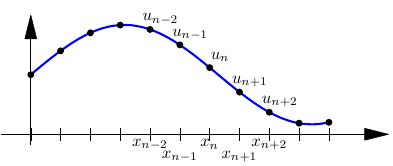
\[\begin{aligned} \frac{d}{dx} u(x_n) \approx \frac{u_{n+2}-8u_{n+1}+8u_{n-1}-u_{n-1}}{12\Delta x} \end{aligned}\]
or one-sided (e.g. for stability, “upwinding”):
\[\begin{aligned} \frac{d}{dx} u(x_n) \approx \frac{3u_n-16u_{n-1}+36u_{n-2}-48u_{n-3}+25u_{n-4}}{25\Delta x} \end{aligned}\]
Simple, efficient, flexible
Needs structured neighborhood of nodes – hard to generalize to unstructured grids in 2-D and 3-D
The Finite Element Method (FEM)
Discretize domain into elements (intervals)
Seek approximate solution in space of piecewise polynomials \(\hat{X}\)
Impose equation weakly: Seek \(\hat{u}\in \hat{X}\) such that for all \(v\in \hat{X}\):
\[\begin{aligned} &\int_0^1 (\hat{u}_t+\hat{u}_x) v\, dx \\ &= \int_0^1 \hat{u}_t v\,dx + \int_0^1 \hat{u}_x v\, dx \\ &= \int_0^1 \hat{u}_t v\,dx - \int_0^1 \hat{u} v_x\, dx = 0 \end{aligned}\]
Leads to semi-discrete system \(M \boldsymbol{u}_t + K\boldsymbol{u} = 0\), with element-wise local \(M,K\) matrices
\(M^{-1}\) dense \(\Longrightarrow\) Explicit methods for \(\boldsymbol{u}_t = -M^{-1}K\boldsymbol{u}\) not practical
Also, unclear how to stabilize by upwinding (but other techniques exist, such as Streamline Upwind Petrov-Galerkin)
The Discontinuous Galerkin Method
Do not enforce continuity – allow “jumps” between elements
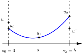
Galerkin formulation for single element \(\kappa=[0,h]\): For all \(v\in P^p(\kappa)\),
\[\begin{aligned} \int_0^h (\hat{u}_t+\hat{u}_x)v\, dx &= \int_0^h \hat{u}_t v\, dx + \int_0^h \hat{u}_x v\, dx \\ &= \int_0^h \hat{u}_t v\, dx - \int_0^h \hat{u}v_x\,dx +\mathcal{U}(u^+,u_p) v(h) - \mathcal{U}(u_0,u^-)v(0) \end{aligned}\]
Numerical flux function \(\mathcal{U}(u_R,u_L)\) allows for stabilization by high-order upwinding, e.g. \(\mathcal{U}(u_R,u_L) = u_L\)
The Discontinuous Galerkin Method
The DG formulation leads to linear system of equations: \[\begin{aligned} M \boldsymbol{u}_t+K\boldsymbol{u} +\begin{pmatrix} -u^- & 0 & \cdots & 0 & u_p \end{pmatrix}^T = 0 \end{aligned}\]
For example, with \(p=2\): \[\begin{aligned} \boldsymbol{u}_t &= -M^{-1} K \boldsymbol{u} - M^{-1} \begin{pmatrix} -u^- & 0 & u_2 \end{pmatrix}^T \\ &= \frac{1}{h} \begin{pmatrix} -6 & -4 & 1 \\ 2.5 & 0 & -1 \\ -4 & 4 & -3 \end{pmatrix} \begin{pmatrix} u_0 \\ u_1 \\ u_2 \end{pmatrix} + \frac{1}{h} \begin{pmatrix} 9 \\ -1.5 \\ 3 \end{pmatrix} u^- \end{aligned}\]
Element-wise local FD-type stencil
Stabilized, “upwinded” through \(u^-\)
Extends naturally to other PDEs, N-D, unstructured meshes
The DG Scheme – Details of Discretization
Consider the 1-D conservation law \[\begin{aligned} \frac{\partial u}{\partial t} + \frac{\partial f(u)}{\partial x} = 0 \end{aligned}\]
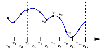
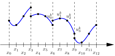
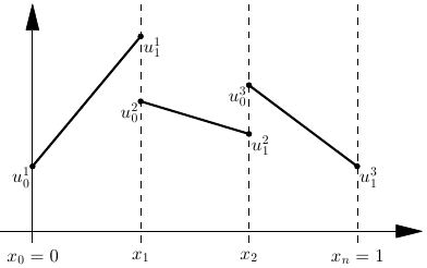
Seek a solution in space of piecewise polynomial functions \(X_h\)
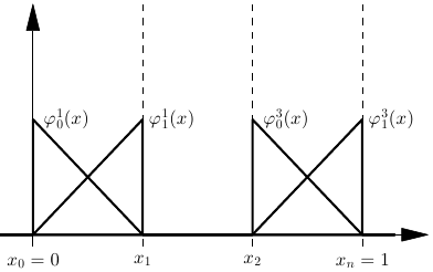
Nodal representation with values \(u_i^k\) for local node \(i\) in element \(k\): \[\begin{aligned} u_h(x) = \sum_{k=1}^n \sum_{i=0}^p u_i^k \phi_i^k(x) \end{aligned}\]
Example, piecewise linear functions (\(p=1\)):
The DG Scheme – Details of Discretization
Galerkin formulation: Find \(u_h\in X_h\) such that \[\begin{aligned} \int_0^1 \frac{\partial u_h}{\partial t}v\, dx + \int_0^1 \frac{\partial f(u_h)}{\partial x}v\,dx = 0 \end{aligned}\]
Set \(v=\phi_i^k\) and integrate by parts \[\begin{aligned} \int_{x_{k-1}}^{x_k} \frac{\partial u_h}{\partial t} \phi_i^k\,dx + \left[ f(u_h(x))\phi_i^k(x) \right]_{x_{k-1}}^{x_k} -\int_{x_{k-1}}^{x_k} f(u_h)\frac{d\phi_i^k}{dx}\,dx = 0 \end{aligned}\]
Use a numerical flux function \(F(u_R,u_L)\) at the discontinuities \[\begin{aligned} &\int_{x_{k-1}}^{x_k} \frac{\partial u_h}{\partial t} \phi_i^k\,dx + F(u_0^{k+1},u_p^k)\phi_i^k(x_k) - F(u_0^k,u_p^{k-1})\phi_i^k(x_k) \\ &-\int_{x_{k-1}}^{x_k} f(u_h)\frac{d\phi_i^k}{dx}\,dx = 0 \end{aligned}\]
The DG Scheme – Details of Discretization
Example: \(f(u)=u\), \(F(u_R,u_L)=u_L\) \[\begin{aligned} &\hspace{-1.2cm}\int_{x_{k-1}}^{x_k} \frac{\partial}{\partial t} \left( \sum_{k=1}^n \sum_{j=0}^p u_j^k \phi_j^k(x) \right) \phi_i^k\,dx - \int_{x_{k-1}}^{x_k} \left( \sum_{k=1}^n \sum_{j=0}^p u_j^k \phi_j^k(x) \right) \frac{d\phi_i^k}{dx}\,dx \\ & +u_p^k\phi_i^k(x_k)-u_p^{k-1}\phi_i^k(x_{k-1}) = 0 \end{aligned}\]
Rearrange to obtain a linear system of equations \[\begin{aligned} M^k \dot{u}^k-C^k u^k + \begin{bmatrix} -u_p^{k-1} & 0 & \cdots & 0 & u_0^k \end{bmatrix}^T = 0 \end{aligned}\] for element \(k\), with elementary matrices \[\begin{aligned} M_{ij}^k = \int_{x_{k-1}}^{x_k} \phi_i^k\phi_j^k\,dx\text{ and } C_{ij}^k = \int_{x_{k-1}}^{x_k} \frac{d\phi_i^k}{dx}\phi_j^k\,dx \end{aligned}\]
Calculating Elementary Matrices
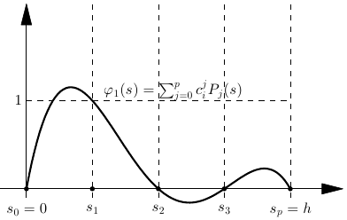
Consider an element of degree \(p\), width \(h\), and a nodal basis at the points \(s_i=h_i/p\), \(i=0,\ldots,p\)
For \(p\) high \((>4)\), use Gauss-Lobatto points instead
Write basis functions in monomial form \(\phi_i(s) = \sum_{j=0}^p c_i^j s^j\)
For \(p\) high \((>4)\), use an orthogonal basis instead
Nodal basis functions are defined by \[\begin{aligned} \phi_i(s_k) = \delta_{ij} = \begin{cases} 1 & i=j \\ 0 & i\ne j \end{cases} \end{aligned}\]
Produces a linear system of equations
Calculating Elementary Matrices
The linear system of equations has the form \[\begin{aligned} \begin{pmatrix} 1 & s_0 & s_0^2 & \cdots & s_0^p \\ 1 & s_1 & s_1^2 & \cdots & s_1^p \\ \vdots & \vdots & \vdots & \ddots & \vdots \\ 1 & s_p & s_p^2 & \cdots & s_p^p \\ \end{pmatrix} \begin{pmatrix} c_0^0 & c_1^0 & \cdots & c_p^0 \\ c_0^1 & c_1^1 & \cdots & c_p^1 \\ \vdots & \vdots & \ddots & \vdots \\ c_0^p & c_1^p & \cdots & c_p^p \\ \end{pmatrix} = \begin{pmatrix} 1 & & & \\ & 1 & & \\ & & \ddots & \\ & & & 1 \end{pmatrix} \end{aligned}\] or \(VC=I\), which gives the coefficient matrix \(C=V^{-1}\)
Use Gaussian quadrature or explicit polynomial integration to compute the elementary matrices \[\begin{aligned} M_{ij}&=\int_0^h \phi_i(s)\phi_j(s)\, ds \\ C_{ij}&=\int_0^h \phi_i'(s)\phi_j(s)\, ds \end{aligned}\]
DG formulations for 1-D Poisson
DG for Elliptic Problems – Historical Overview
Enforcing Dirichlet conditions by penalties
Lions (1968), Babuška (1973) – Penalty term
Nitsche (1971) – additional terms in bilinear form for consistency
Interior Penalty (IP) methods
Babuška and Zlámal (1973) – enforce \(C^1\)-continuity by penalties
Wheeler (1978), Arnold (1979) – Nitsche’s method for spaces of discontinuous piecewise polynomials
DG methods
Bassi and Rebay (1997) – apply RKDG to unknown and its gradient
Cockburn and Shu (1998) – generalized the ideas, the LDG method
Unification
Arnold, Brezzi, Cockburn, Marini (2000,2002) – showed that most methods fit in a unified framework by choosing appropriate numerical fluxes
Second-order Equations
Consider the 1-D Poisson equation \[\begin{aligned} -\frac{d ^2 u}{d x ^2} = f(x)\quad\text{ in } [0,1] \end{aligned}\] with homogeneous Dirichlet conditions \(u(0)=u(1)=0\)
Standard Continuous Galerkin FEM would consider the space \(X_{h,0}\) of continuous piecewise polynomials satisfying the Dirichlet conditions, and solve for \(u_h \in X_{h,0}\) s.t. \[\begin{aligned} \int_0^1 -\frac{d^2u_h}{dx^2} v \,dx = \int_0^1 \frac{du_h}{dx} \frac{dv}{dx}\,dx - \left[\frac{du_h}{dx} v\right]_0^1 = \int_0^1 \frac{du_h}{dx} \frac{dv}{dx}\,dx = \int_0^1 f\,v\,dx \end{aligned}\] for all \(v\in X_{h,0}\)
With discontinuous functions, appropriate numerical fluxes must be chosen at all element boundaries
The 1-D Poisson Equation
To define a DG discretization, first split into first order system: \[\begin{aligned} -\sigma'=f(x),\quad u'=\sigma \end{aligned}\]
Multiply by test functions \(v,\tau\), integrate over an element, and integrate by parts to obtain the weak form \[\begin{aligned} \int_{x_k}^{x_{k+1}} f(x)\,v\,dx &= \int_{x_k}^{x_{k+1}} -\sigma' v\,dx = \int_{x_k}^{x_{k+1}} \sigma v'\,dx -\left[\hat{\sigma} v\right]_0^1 \\ \int_{x_k}^{x_{k+1}} \sigma\,\tau\,dx &= \int_{x_k}^{x_{k+1}} u'\,\tau\,dx = -\int_{x_k}^{x_{k+1}} u\,\tau'\,dx + \left[ \hat{u} \tau \right]_0^1 \end{aligned}\]
Galerkin formulation: Find \(u_h,\sigma_h\in X_h\) s.t. for all elements \(k\) \[\begin{aligned} \int_{x_k}^{x_{k+1}} \sigma_h v'\,dx &= \int_{x_k}^{x_{k+1}} f(x)\,v\,dx + \left[\hat{\sigma}(u_h,\sigma_h) v\right]_0^1, && \forall v\in X_h \\ \int_{x_k}^{x_{k+1}} \sigma_h\,\tau\,dx &= -\int_{x_k}^{x_{k+1}} u_h\,\tau'\,dx + \left[ \hat{u}(u_h) \tau \right]_0^1, && \forall \tau\in X_h \end{aligned}\]
Remains only to define the numerical fluxes \(\hat{u}(u_h),\hat{\sigma}(u_h,\sigma_h)\)
The BR1 Fluxes
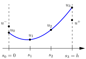
The BR1 fluxes: \[\begin{aligned} \hat{u}=\{ u_h \},\qquad \hat{\sigma} = \{ \sigma_h \} \end{aligned}\] where \(\{\cdot\}\) is the averaging operator
For example, with notation according to the figure: \[\begin{aligned} \hat{u}(0) &= (u^-+u_0)/2\text{\ \ and\ \ }\hat{u}(h) = (u_3+u^+)/2 \\ \hat{\sigma}(0) &= (\sigma^-+\sigma_0)/2\text{\ \ and\ \ }\hat{\sigma}(h) = (\sigma_3+\sigma^+)/2 \end{aligned}\]
Simple, intuitive (no preference to direction in equation)
However, unstable and non-compact stencil
Interior Penalty (IP)
In the interior penalty method, we set \[\begin{aligned} \hat{u}&=\{ u_h \} \\ \hat{\sigma} &= \{ \nabla u_h \} + C_{11} \left[\left[\right.\right.u_h \left.\left.\right]\right] \end{aligned}\]
for some \(C_{11}>0\), where \(\{\cdot\}\) is the averaging operator and \(\left[\left[\right.\right.\cdot \left.\left.\right]\right]\) is the jump operator
For example, with notation according to the figure: \[\begin{aligned} \hat{u}(0) &= (u^-+u_0)/2\text{\ \ and\ \ }\hat{u}(h) = (u_3+u^+)/2 \\ \hat{\sigma}(0) &= (\left.u_h'\right|_{x=0^-} + \left.u_h'\right|_{x=0^+})/2 + C_{11} (u^- - u_0) \\ \hat{\sigma}(h) &= (\left.u_h'\right|_{x=h^-} + \left.u_h'\right|_{x=h^+})/2 + C_{11} (u_3-u^+) \end{aligned}\]
Convergent with optimal order of accuracy
However, \(C_{11}\) is problem dependent, introduces stiffness
The Local Discontinuous Galerkin (LDG) Method
In the LDG method, we set \[\begin{aligned} \hat{u}&=\{ u_h \} + C_{12} \left[\left[\right.\right.u_h \left.\left.\right]\right]\\ \hat{\sigma} &= \{ \sigma_h \} + C_{11} \left[\left[\right.\right.u_h \left.\left.\right]\right]-C_{12} \left[\left[\right.\right.\sigma_h \left.\left.\right]\right] \end{aligned}\]
For the special cases \(C_{11}=0\) (minimal dissipation LDG) and \(C_{12}=1/2\) we get a simple upwind/downwind structure
For example, with notation according to the figure: \[\begin{aligned} \hat{u}(0) &= u_0 \text{\ \ and\ \ }\hat{u}(h) = u^+ \\ \hat{\sigma}(0) &= \sigma^- \text{\ \ and\ \ }\hat{\sigma}(h) = \sigma_3 \end{aligned}\]
Simple and general
Convergent with optimal order of accuracy
However, in general a non-compact stencil in higher dimensions
The Local Discontinuous Galerkin (LDG) Method
The LDG Method
In the LDG method, we use the fluxes \[\begin{aligned} \hat{\sigma}_K &= \{\sigma_h\} + C_{11} \left[\left[\right.\right.u_h \left.\left.\right]\right]- \boldsymbol{C}_{12} \left[\left[\right.\right.\sigma_h \left.\left.\right]\right]\\ \hat{u}_K &= \{u_h\} +\boldsymbol{C}_{12} \cdot \left[\left[\right.\right.u_h \left.\left.\right]\right] \end{aligned}\]
Here, \(C_{11}>0\) (or zero for the minimal dissipation LDG method, Cockburn and Dong 2007)
An important special case for \(\boldsymbol{C}_{12}\) is the choice \[\begin{aligned} \boldsymbol{C}_{12} = \frac12 (S_{K^+}^{K^-1} n^+ + S_{K^-}^{K^+} n^- ) \end{aligned}\] where \(S_{K^+}^{K^-}\in\{0,1\}\) is a switch for the edge shared by \(K^-\) and \(K^+\)
This leads to a simple upwind/downwind scheme: \[\begin{aligned} \hat{\sigma}_K = C_{11} \left[\left[\right.\right.u_h \left.\left.\right]\right]+ \begin{cases} \sigma_h^+ & \text{if }S_{K^+}^{K^-}=0 \\ \sigma_h^- & \text{if }S_{K^+}^{K^-}=1 \end{cases}, \qquad \hat{u}_K = \begin{cases} u_h^- & \text{if }S_{K^+}^{K^-}=0 \\ u_h^+ & \text{if }S_{K^+}^{K^-}=1 \end{cases} \end{aligned}\]
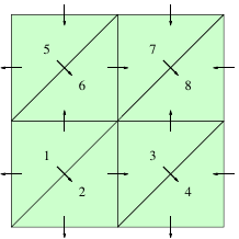
LDG Switch Functions
Natural switch: Order the elements, let \(N_K\) be the index of element \(K\), and set \[\begin{aligned} S_{K^+}^{K^-} = 1 \text{ if } N_{K^+}>N_{K^-},\quad 0 \text{ otherwise}. \end{aligned}\] Simple, leads to beneficial matrix structure, but unstable if \(C_{11}=0\) in the original LDG method
Consistent switch: For example define any constant vector \(\beta\) and set \[\begin{aligned} S_{K^+}^{K^-} = 1 \text{ if } n^+ \cdot \beta>0,\quad 0 \text{ otherwise}. \end{aligned}\]
In general, any choice of switch leads to a non-compact stencil
Natural switch
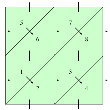
Consistent switch
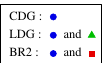
The Compact Discontinuous Galerkin (CDG) Method
The Compact DG (CDG) Method
To address the non-compactness of the LDG method and its sensitivity to the switch, Peraire and Persson developed the Compact DG method (2008)
Recall the original LDG fluxes: \[\begin{aligned} \hat{\sigma}_K &= \{\sigma_h\} + C_{11} \left[\left[\right.\right.u_h \left.\left.\right]\right]- \boldsymbol{C}_{12} \left[\left[\right.\right.\sigma_h \left.\left.\right]\right]\\ \hat{u}_K &= \{u_h\} +\boldsymbol{C}_{12} \cdot \left[\left[\right.\right.u_h \left.\left.\right]\right] \end{aligned}\]
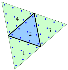
Now, introduce the edge fluxes \(\sigma_h^e\) on edge \(e\) by \[\begin{aligned} \int_K \sigma_h^e\cdot\tau\,dx &= -\int_K u_h \nabla\cdot\tau\,dx + \int_{\partial K} \hat{u}^e_K\,n_K\cdot\tau\,ds, && \forall\tau\in[\mathcal{P}_p(K)]^2 \end{aligned}\]
where \[\begin{aligned} \hat{u}^e_K = \begin{cases} \hat{u}_K & \text{on edge }e\text{, as defined above} \\ u_h & \text{otherwise} \end{cases} \end{aligned}\]
The Compact DG (CDG) Method
The numerical fluxes for CDG are then simply given by \[\begin{aligned} \hat{\sigma}^e_K &= \{\sigma_h^e\} + C_{11} \left[\left[\right.\right.u_h \left.\left.\right]\right]- \boldsymbol{C}_{12} \left[\left[\right.\right.\sigma_h^e \left.\left.\right]\right] \end{aligned}\] on edge \(e\)
The modification eliminates the non-compact terms in the primal form, while retaining all the good properties of the LDG scheme
In addition, better stability properties are observed with in particular less sensitivity to the choice of switch function
The CDG Method – Summary
Element-wise compact stencil
Less connectivities than LDG/BR2/IP
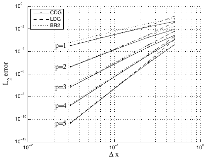
More accurate than LDG and BR2
Properties of the CDG Method
Switches and Null-space Dimensions
Unlike the LDG scheme, the CDG scheme appears to be stable for \(C_{11}=0\) and an inconsistent switch such as highest element number
Simple test [Sherwin et al 05]: Poisson problem, periodic boundary conditions, expected nullspace dimension = 1
Nullspace dimension
| Polynomial order \(p\) | \(1\) | \(2\) | \(3\) | \(4\) | \(5\) | \(6\) | \(7\) | |
|---|---|---|---|---|---|---|---|---|
| Consistent switch | CDG | \(1\) | \(1\) | \(1\) | \(1\) | \(1\) | \(1\) | \(1\) |
| LDG | \(1\) | \(1\) | \(1\) | \(1\) | \(1\) | \(1\) | \(1\) | |
| Natural switch | CDG | \(1\) | \(1\) | \(1\) | \(1\) | \(1\) | \(1\) | \(1\) |
| LDG | \(3\) | \(4\) | \(5\) | \(6\) | \(7\) | \(8\) | \(9\) |
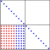
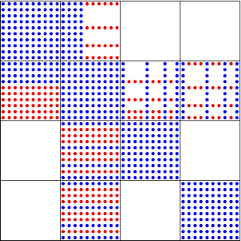
ILU and Switch Orientation
Orientation of lower-triangular blocks important for ILU sparsity
Take advantage of CDG’s insensitivity to orientation
 \(A\)
\(A\)
\(=\)
 \(L\)
\(L\)
 \(U\)
\(U\)
Switch 1:
Same LU storage
 \(A\)
\(A\)
\(=\)
 \(L\)
\(L\)
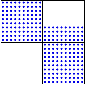 \(U\)
\(U\)
Switch 2:
More LU storage
Switches and Null-space Dimensions
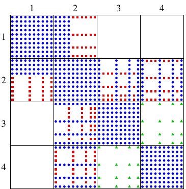
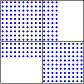
No additional non-zeros in block-ILU(0) factorization using CDG
Dense lower-triangular blocks using BR2 / IP
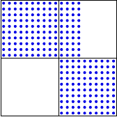
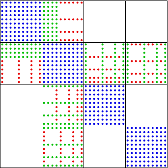
CDG
Stiffness Matrix
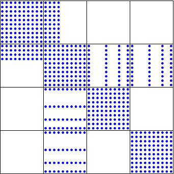
640 non-zeros
Block ILU(0)
640 non-zeros
Switches and Null-space Dimensions
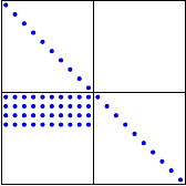
No additional non-zeros in block-ILU(0) factorization using CDG
Dense lower-triangular blocks using BR2 / IP
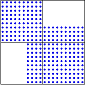
BR2 / IP
Stiffness Matrix
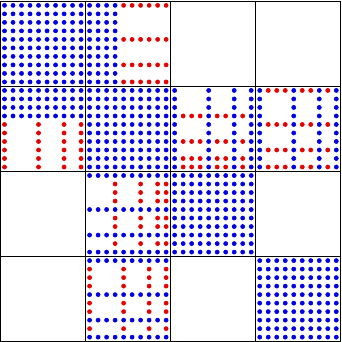
784 non-zeros
Block ILU(0)
892 non-zeros
Matrix Representation
Block matrix representation fundamental for high performance
Solver algorithms based on blocks
Up to 10 times higher performance with optimized BLAS
Compact stencil \(\Longrightarrow\) Matrix structure given by mesh connectivities
Hard to store LDG/BR2/IP efficiently

CDG – 2 arrays
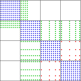
LDG – 3 arrays + struct
BR2 / IP – 3 arrays