Introduction to FEM

A simple example

Consider the model problem \[\begin{aligned} -u''(x) &= 1,\text{ for } x\in (0,1) \label{model1eq1} \\ u(0) &= u(1) = 0 \label{model1eq2} \end{aligned}\] with exact solution \(u(x) = x(1-x)/2\). Find an approximate solution of the form \[\begin{aligned} \hat{u}(x) = A \sin (\pi x) = A \varphi(x) \end{aligned}\] Various ways to impose the equation:

Collocation

: Impose \(-\hat{u}''(x_c) = 1\) for some collocation point \(x_c\) \(\Longrightarrow\) \(A\pi^2\sin(\pi x_c) = 1\)

• \(x_c=\frac12\) \(\Longrightarrow\) \(A= \frac{1}{\pi^2} = 0.1013\)

• \(x_c=\frac14\) \(\Longrightarrow\) \(A= \frac{\sqrt{2}}{\pi^2} = 0.1433\)

Average

: Impose the average of the equation over the interval: \[\begin{aligned} \int_0^1 -\hat{u}''(x)\,dx &= \int_0^1 1\,dx \\ \int_0^1 A\pi^2 \sin(\pi x)\,dx &= A\pi^2 \frac{2}{\pi} = 2A\pi = 1 \\ A &= \frac{1}{2\pi} = 0.159 \end{aligned}\]

Galerkin

: Impose the weighted average of the equation over the interval: \[\begin{aligned} \int_0^1 -\hat{u}''(x) v(x)\,dx = \int_0^1 1\cdot v(x)\,dx \end{aligned}\] A Galerkin method using the weight functions \(v(x)\) from the same space as the solution space, that is, \(v(x) = \varphi(x)\). This gives \[\begin{aligned} \int_0^1 A\pi^2 \sin^2(\pi x)\, dx &= \int_0^1 \sin(\pi x)\, dx \\ A\pi^2 \cdot \frac12 &= \frac{2}{\pi} \\ A &= \frac{4}{\pi^3} = 0.129 \end{aligned}\]

The three solutions are shown in figure 1. The finite element method is based on the Galerkin formulation, which in this example clearly is superior to collocation or averaging.

Solutions of the model problem ([model1eq1])-([model1eq2]) using collocation, average, and Galerkin.

Other function spaces

Use piecewise linear, continuous functions of the form \(\hat{u}(x) = A\varphi(x)\) with \[\begin{aligned} \varphi(x) = \begin{cases} 2x & x\le \frac12 \\ 2-2x & x>\frac12 \end{cases} \end{aligned}\] Galerkin gives the FEM formulation \[\begin{aligned} \int_0^1 -\hat{u}''(x) \varphi(x)\,dx = \int_0^1 \varphi(x)\,dx \end{aligned}\] Since \(\hat{u}''\) is not bounded, integrate LHS by parts: \[\begin{aligned} \int_0^1 \hat{u}'(x) \varphi'(x)\, dx - \left[ \hat{u}'(x) \varphi(x) \right]_0^1 &= \int_0^1 \hat{u}'(x) \varphi'(x)\, dx - \hat{u}'(1)\varphi(1) + \hat{u}'(0)\varphi(0) \\ &= \int_0^1 \hat{u}'(x) \varphi'(x)\, dx, \end{aligned}\] since \(\varphi(0)=\varphi(1)=0\). This leads to the final formulation \[\begin{aligned} \int_0^1 \hat{u}'(x)\varphi'(x)\,dx = \int_0^1 \varphi(x)\,dx. \label{model1fem} \end{aligned}\] To solve for \(\hat{u}(x)=A\varphi(x)\), note that \(\hat{u}'(x)=A\varphi'(x)\) and \[\begin{aligned} \varphi'(x) = \begin{cases} 2 & x\le \frac12 \\ -2 & x>\frac12 \end{cases} \end{aligned}\] Equation ([model1fem]) then becomes \[\begin{aligned} \int_0^{1/2} (2A)(2)\,dx + \int_{1/2}^1 (-2A)(-2)\,dx &= \int_0^{1/2} 2x\,dx + \int_{1/2}^1 (2-2x)\,dx \end{aligned}\] or \(4A = 1/2\), that is, \(A = 1/8\), and the FEM solution is \(\hat{u}(x) = \varphi(x)/8\).

More basis functions

To refine the solution space, introduce a triangulation of the domain \(\Omega=[0,1]\) into non-overlapping elements: \[\begin{aligned} T_h = \{K_1,K_2,\ldots \} \end{aligned}\] such that \(\Omega = \cup_{K\in T_h} K\). Now consider the space of continuous functions that are piecewise linear on the triangulation and zero at the end points: \[\begin{aligned} V_h = \{ v\in C^0([0,1]) : v|_K \in \mathbb{P}_1(K)\ \forall K\in T_h,\ v(0)=v(1)=0 \}. \end{aligned}\] Here \(\mathbb{P}_p(K)\) is the space of polynomials on \(K\) of degree at most \(p\). Define a basis \(\{\varphi_i\}\) for \(V_h\) by the basis functions \(\varphi_i\in V_h\) with \(\varphi_i(x_j) = \delta_{ij}\), for \(i,j=1,\ldots,n\). Our approximate solution \(u_h(x)\) can then be written in terms of its expansion coefficients and the basis functions as \[\begin{aligned} u_h(x) = \sum_{i=1}^n u_i \varphi_i(x), \label{femsol} \end{aligned}\] where we note that this particular basis has the convenient property that \(u_h(x_j) = u_j\), for \(j=1,\ldots,n\).

A refined piecewise linear function space, same solution and basis functions.

A Galerkin formulation for ([model1eq1])-([model1eq2]) can now be stated as: Find \(u_h\in V_h\) such that \[\begin{aligned} \int_0^1 u'_h(x) v'(x)\,dx = \int_0^1 v(x)\,dx,\qquad \forall v\in V_h \label{modelgal1} \end{aligned}\] In particular, ([modelgal1]) should be satisfied for \(v=\varphi_i\), \(i=1,\ldots,n\), which leads to \(n\) equations of the form \[\begin{aligned} \int_0^1 u'_h(x) \varphi_i'(x)\,dx = \int_0^1 \varphi_i(x)\,dx,\qquad \text{for } i=1,\ldots,n \end{aligned}\] Insert the expression ([femsol]) for the approximate solution and its derivative, \(u'_h(x) = \sum_{i=1}^n u_i \varphi'_i(x)\): \[\begin{aligned} \int_0^1 \left( \sum_{j=1}^n u_j \varphi'_j(x) \right) \varphi'_i(x)\,dx &= \int_0^1 \varphi_x(x)\,dx,\qquad i=1,\ldots,n \end{aligned}\] Change order of integration/summation: \[\begin{aligned} \sum_{j=1}^n u_j \left[ \int_0^1 \varphi'_i(x) \varphi'_j(x)\,dx \right] &= \int_0^1 \varphi_i(x)\,dx,\qquad i=1,\ldots,n \end{aligned}\] This is a linear system of equations \(A\boldsymbol{u} = \boldsymbol{f}\), with \(A=[ a_{ij} ]\), \(\boldsymbol{u} = [ u_i ]\), \(\boldsymbol{f} = [ f_i ]\), for \(i,j=1,\ldots,n\), where \[\begin{aligned} a_{ij} &= \int_0^1 \varphi'_i(x) \varphi'_j(x)\,dx \\ f_i &= \int_0^1 \varphi_i(x)\,dx \end{aligned}\]

Example

: Consider a triangulation of \([0,1]\) into four elements of width \(h=1/4\) between the node points \(x_i = ih\), \(i=0,\ldots,4\). We then get a solution space of dimension \(n=3\), and basis functions \(\varphi_1,\varphi_2,\varphi_3\). When calculating the entries of \(A\), note that

• \(A\) is symmetric, that is, \(a_{ij} = a_{ji}\)

• \(A\) is tridiagonal, that is, \(a_{ij}=0\) whenever \(|i-j|>1\)

• For our equidistant triangulation, \(a_{ii} = a_{jj}\) and \(a_{i,i+1} = a_{j,j+1}\)

This gives \[\begin{aligned} a_{11} &= 4\cdot 4 \cdot \frac14 + (-4)(-4)\frac14 = 8 \\ a_{12} &= (-4)\cdot 4 \cdot \frac14 = -4 \\ a_{22} &= a_{33} = a_{11} = 8 \\ a_{21} &= a_{12} = a_{23} = a_{32} = -4 \\ a_{13} &= a_{31} = 0 \end{aligned}\] and \[\begin{aligned} f_1 &= f_2 = f_3 = \int_0^1 \varphi_1(x)\,dx = \frac14 \end{aligned}\] and the linear system becomes \[\begin{aligned} \begin{bmatrix} 8 & -4 & 0 \\ -4 & 8 & -4 \\ 0 & -4 & 8 \end{bmatrix} \begin{bmatrix} u_1 \\ u_2 \\ u_3 \end{bmatrix} = \begin{bmatrix} 1/4 \\ 1/4 \\ 1/4 \end{bmatrix} \end{aligned}\] with solution \[\begin{aligned} u = (u_1, u_2, u_3)^T = (3/32, 1/8, 3/32)^T \end{aligned}\] Note that the discretization exactly matches the one obtained with finite differences and the 2nd order 3-point stencil: \[\begin{aligned} \frac{1}{(1/4)^2} \begin{bmatrix} 2 & -1 & 0 \\ -1 & 2 & -1 \\ 0 & -1 & 2 \end{bmatrix} \begin{bmatrix} u_1 \\ u_2 \\ u_3 \end{bmatrix} = \begin{bmatrix} 1 \\ 1 \\ 1 \end{bmatrix} \end{aligned}\]

Neumann boundary conditions

The Dirichlet conditions \(u(0)=u(1)=0\) where enforced directly into the approximation space \(V_h\). In the finite element method, a Neumann condition (or natural condition) is instead implemented by modifying the variational formulation. Consider the model problem \[\begin{aligned} -u''(x) &= f(x)\text{ for } x\in(0,1) \\ u(0) &= 0 \\ u'(1) &= g \end{aligned}\] The function space is only enforcing the Dirichlet condition at the left end point: \[\begin{aligned} V_h = \{ v\in C^0([0,1]) : v|_K \in \mathbb{P}_1(K)\ \forall K\in T_h,\ v(0)=0 \}, \end{aligned}\] which in our example gives an additional degree of freedom. The Neumann condition appears in the formulation after integration by parts: \[\begin{aligned} \int_0^1 \hat{u}'(x) v'(x)\, dx - \left[ \hat{u}'(x) v(x) \right]_0^1 &= \int_0^1 \hat{u}'(x) v'(x)\, dx - \hat{u}'(1)v(1) + \hat{u}'(0)v(0) \\ &= \int_0^1 \hat{u}'(x) v'(x)\, dx - gv(1) \end{aligned}\] since \(v(0)=0\) and \(u'_h(1)=g\). This leads to the final formulation: Find \(u_h\in V_h\) such that \[\begin{aligned} \int_0^1 u'_h(x) v'(x)\,dx = \int_0^1 f(x) v(x)\,dx + gv(1),\qquad \forall v\in V_h \label{modelgal2} \end{aligned}\]

Example

: With our previous triangulation, we now get another basis function \(\varphi_4\). For simplicity, set \(f=g=1\). All the matrix entries and right-hand side values are then identical, and we only calculate the new values: \[\begin{aligned} a_{44} &= (4)^2 \frac14 = 4 \\ a_{34} &= a_{43} = (-4)\cdot 4 \cdot \frac14 = -4 \\ f_4 &= \frac18 + g\cdot 1 = \frac98 \end{aligned}\] The linear system then becomes \[\begin{aligned} \begin{bmatrix} 8 & -4 & 0 & 0\\ -4 & 8 & -4 & 0\\ 0 & -4 & 8 & -4 \\ 0 & 0 & -4 & 4 \end{bmatrix} \begin{bmatrix} u_1 \\ u_2 \\ u_3 \\ u_4 \end{bmatrix} = \begin{bmatrix} 1/4 \\ 1/4 \\ 1/4 \\ 9/8 \end{bmatrix} \end{aligned}\] with solution \[\begin{aligned} u = (u_1, u_2, u_3, u_4)^T = (15/32, 7/8, 39/32, 3/2)^T. \end{aligned}\]

Inhomogeneous Dirichlet problems

Use two spaces: \(V_h\), which enforces the inhomogeneous Dirichlet condition, for the solution \(u_h\), and \(V^0_h\), which enforces homogeneous Dirichlet conditions, for the test function \(v\). Consider for example the model problem \[\begin{aligned} -u''(x) &= f,\text{ for } x\in (0,1) \label{model2eq1} \\ u(0) &= 0 \label{model2eq2} \\ u(1) &= 1 \label{model2eq3} \end{aligned}\] with exact solution \(u(x) = x(3-x)/2\). Use the spaces \[\begin{aligned} V_h = \{ v\in C^0([0,1]) : v|_K \in \mathbb{P}_1(K)\ \forall K\in T_h,\ v(0)=0, v(1)=1 \}, \\ V^0_h = \{ v\in C^0([0,1]) : v|_K \in \mathbb{P}_1(K)\ \forall K\in T_h,\ v(0)=0, v(1)=0 \}. \end{aligned}\] The FEM formulation becomes: Find \(u_h\in V_h\) such that \[\begin{aligned} \int_0^1 u_h' v'\,dx = \int_0^1 fv\, dx,\qquad \forall v\in V^0_h. \end{aligned}\] Note that the function space \(V_h\) is not a linear vector space, due to the inhomogeneous constraint. In practice, Dirichlet conditions are implemented by first considering the all-Neumann problem, and enforcing the Dirichlet conditions directly into the resulting system of equations.

Example

: For the model problem ([model2eq1])-([model2eq3]), first consider the corresponding all-Neumann problem \[\begin{aligned} -u''(x) &= f,\text{ for } x\in (0,1) \label{model2neueq1} \\ u'(0) &= u'(1) = 0 \label{model2neueq2} \end{aligned}\] with the solution space \[\begin{aligned} V_h = \{ v\in C^0([0,1]) : v|_K \in \mathbb{P}_1(K)\ \forall K\in T_h \}. \end{aligned}\] In our example with four elements of size \(h=1/4\), this gives \(5\) degrees of freedom and the resulting linear system (with \(f=1\)): \[\begin{aligned} \begin{bmatrix} 4 & -4 & 0 & 0 & 0 \\ -4 & 8 & -4 & 0 & 0\\ 0 & -4 & 8 & -4 & 0\\ 0 & 0 & -4 & 8 & -4 \\ 0 & 0 & 0 & -4 & 4 \end{bmatrix} \begin{bmatrix} u_1 \\ u_2 \\ u_3 \\ u_4 \\ u_5 \end{bmatrix} = \begin{bmatrix} 1/8 \\ 1/4 \\ 1/4 \\ 1/4 \\ 1/8 \end{bmatrix} \end{aligned}\] This system is singular (since the solution is undetermined up to a constant). We can now impose the Dirichlet conditions \(u(0)=0\) and \(u(1)=1\) directly by replacing the corresponding equations: \[\begin{aligned} \begin{bmatrix} 1 & 0 & 0 & 0 & 0 \\ -4 & 8 & -4 & 0 & 0\\ 0 & -4 & 8 & -4 & 0\\ 0 & 0 & -4 & 8 & -4 \\ 0 & 0 & 0 & 0 & 1 \end{bmatrix} \begin{bmatrix} u_1 \\ u_2 \\ u_3 \\ u_4 \\ u_5 \end{bmatrix} = \begin{bmatrix} 0 \\ 1/4 \\ 1/4 \\ 1/4 \\ 1 \end{bmatrix} \end{aligned}\] We can keep the symmetry of the matrix by eliminating the entries below/above the diagonal of the Dirichlet variables: \[\begin{aligned} \begin{bmatrix} 1 & 0 & 0 & 0 & 0 \\ 0 & 8 & -4 & 0 & 0\\ 0 & -4 & 8 & -4 & 0\\ 0 & 0 & -4 & 8 & 0 \\ 0 & 0 & 0 & 0 & 1 \end{bmatrix} \begin{bmatrix} u_1 \\ u_2 \\ u_3 \\ u_4 \\ u_5 \end{bmatrix} = \begin{bmatrix} 0 \\ 1/4 - (-4)\cdot 0 \\ 1/4 \\ 1/4 - (-4)\cdot 1 \\ 1 \end{bmatrix} = \begin{bmatrix} 0 \\ 1/4 \\ 1/4 \\ 17/4 \\ 1 \end{bmatrix} \end{aligned}\] with solution \(u=(u_1,\ldots,u_5)^T = (0, 11/32, 5/8, 27/32, 1)^T\). If necessary, the Dirichlet degress of freedom can be removed from the system, to obtain the smaller system of equations \[\begin{aligned} \begin{bmatrix} 8 & -4 & 0\\ -4 & 8 & -4\\ 0 & -4 & 8 \\ \end{bmatrix} \begin{bmatrix} u_2 \\ u_3 \\ u_4 \end{bmatrix} = \begin{bmatrix} 1/4 \\ 1/4 \\ 17/4 \end{bmatrix} \end{aligned}\]

The stamping method (“Assembly”)

Consider a single element \(e_k\), and its local basis functions \(\mathcal{H}^k_i(x)\), \(j=1,2\), given by the restriction of the global basis functions \(\varphi_j(x)\) to the element. The connection between the local indices \(i\) and the global indices \(j\) are given by a mesh representation. For simplex elements, we use the form

• \(p\): \(N\times D\) node coordinates

• \(t\): \(T\times (D+1)\) element indices

Here, row \(k\) of \(t\) is the local-to-global mapping for element \(k\). The local basis functions are:

• Defined only inside the element \(e_k\)

• Polynomials of degree 1

We can then define an elemental matrix \(A^k\), or a local stiffness matrix, by again considering only the contribution to the global stiffmatrix from element \(e_k\): \[\begin{aligned} A^k_{ij} = \int_{e_k} (\mathcal{H}^k_i)' \cdot (\mathcal{H}^k_j)'\, dx,\qquad i=1,2,\ j=1,2 \end{aligned}\] and, similarily, an elemental load vector \(\boldsymbol{b}^k\) by \[\begin{aligned} b^k_i = \int_{e_k} f(x)\cdot(\mathcal{H}^k_i)\,dx,\qquad i=1,2 \end{aligned}\]

In the so-called stamping method, or the assembly process, each element matrix and load vector are added at the corresponding global position in the global stiffness matrix and right-hand side vector:

Example

: Equidistant 1D mesh, element width \(h\), piece-wise linears, \(f=1\). The elemental matrix and load vector are \[\begin{aligned} A^k = \frac{1}{h} \begin{bmatrix} 1 & -1 \\ -1 & 1 \end{bmatrix}, \qquad \boldsymbol{b}^k = \frac{h}{2} \begin{bmatrix} 1 \\ 1 \end{bmatrix} \end{aligned}\] The mesh is represented by the arrays \[\begin{aligned} p = \begin{bmatrix} x_0 \\ x_1 \\ \vdots \\ x_n \end{bmatrix}, \qquad t = \begin{bmatrix} 1 & 2 \\ 2 & 3 \\ \vdots \\ n & n+1 \end{bmatrix} \end{aligned}\] The stamping method gives the global matrices: \[\begin{aligned} \frac{1}{h} \begin{bmatrix} 1 & -1 & & & & & \\ -1 & 1 & & & & & \\ \\ \\ \\ \\ \end{bmatrix} &\rightarrow \frac{1}{h} \begin{bmatrix} 1 & -1 & & & & & \\ -1 & 2 & -1& & & & \\ & -1 & 1 \\ \\ \\ \\ \end{bmatrix} \rightarrow \frac{1}{h} \begin{bmatrix} 1 & -1 & & & & & \\ -1 & 2 & -1& & & & \\ & -1 & 2 & -1 \\ & & -1 & 1 \\ \\ \\ \\ \end{bmatrix} \nonumber \\ &\rightarrow \frac{1}{h} \begin{bmatrix} 1 & -1 & & & & & \\ -1 & 2 & -1& & & & \\ & -1 & 2 & -1 \\ & & -1 & 2 & -1 \\ & & & -1 & 2 & -1 \\ & & & & -1 & 2 & -1 \\ & & & & & -1 & 1 \\ \end{bmatrix} = A \end{aligned}\] and, similarily, the right-hand side vector \[\begin{aligned} \boldsymbol{b} = \frac{h}{2} \begin{bmatrix} 1 & 2 & \cdots & 2 & 1 \end{bmatrix}^T \end{aligned}\]

Higher order

Introduce the space of continuous piece-wise quadratics: \[\begin{aligned} V_h = \{ v\in C^0(\Omega) : v|_K \in \mathbb{P}_2(K)\ \forall K\in T_h \}. \end{aligned}\] Parameterize by adding degrees of freedom at element midpoints. Each element then has three local nodes: \(x^k_1, x^k_2, x^k_3\), and three local basis functions \(\mathcal{H}^k_1(x), \mathcal{H}^k_2(x), \mathcal{H}^k_3(x)\). These are determined by solving for the polynomial coefficients in \[\begin{aligned} \mathcal{H}_i^k = a_i + b_ix + c_i x^2,\qquad i=1,2,3 \end{aligned}\] and requiring that \(\mathcal{H}_i^k(x_j) = \delta_{ij}\), for each \(i,j = 1,2,3\). The leads to the linear system of equations \(VC=I\): \[\begin{aligned} \begin{bmatrix} 1 & x_1 & x_1^2 \\ 1 & x_2 & x_2^2 \\ 1 & x_3 & x_3^2 \end{bmatrix} \begin{bmatrix} a_1 & a_2 & a_3 \\ b_1 & b_2 & b_3 \\ c_1 & c_2 & c_3 \end{bmatrix} = \begin{bmatrix} 1 & 0 & 0 \\ 0 & 1 & 0 \\ 0 & 0 & 1 \end{bmatrix} \end{aligned}\] which gives the coefficients \(C = V^{-1}\). For example, with \(x_1=0\), \(x_2=h/2\), \(x_3=h\), we get \[\begin{aligned} \mathcal{H}_1(x) &= \frac{2}{h^2} (x-\frac{h}{2})(x-h) \\ \mathcal{H}_2(x) &= -\frac{4}{h^2} x (x-h) \\ \mathcal{H}_3(x) &= \frac{2}{h^2} x (x-\frac{h}{2}) \end{aligned}\] The corresponding element matrix and the element load can then be calculated as before: \[\begin{aligned} A_{ij}^k = \int_0^h \mathcal{H}_i^k(x)'\mathcal{H}_j^k(x)'\,dx,\qquad b_i^k = \int_0^h f(x) \mathcal{H}_i^k(x)\, dx \end{aligned}\] for \(i,j=1,2,3\), which gives \[\begin{aligned} A^k = \frac{1}{3h} \begin{bmatrix} 7 & -8 & 1 \\ -8 & 16 & -8 \\ 1 & -8 & 7 \end{bmatrix} ,\qquad \boldsymbol{b}^k = \frac{h}{6} \begin{bmatrix} 1 \\ 4 \\ 1 \end{bmatrix} \end{aligned}\] For a global element with two elements of width \(h\), the stamping method gives the stiff matrix and right-hand side vector \[\begin{aligned} A = \frac{1}{3h} \begin{bmatrix} 7 & -8 & 1 \\ -8 & 16 & -8 \\ 1 & -8 & 7+7 & -8 & 1 \\ & & -8 & 16 & -8 \\ & & 1 & -8 & 7 \end{bmatrix},\qquad \boldsymbol{b} = \frac{h}{6} \begin{bmatrix} 1 \\ 4 \\ 1+1 \\ 4 \\ 1 \end{bmatrix} \end{aligned}\]

Numerical Quadrature

For more general cases, the integrals cannot be computed analytically. We then use Gaussian quadrature rules of the following form (not necessarily the same \(f\) as above): \[\begin{aligned} \int_{-1}^1 f(x)\,dx \approx \sum_{i=1}^n w_i f(x_i) \label{gaussquad} \end{aligned}\] when \(x_i,w_i\), \(i=1,\ldots,n\) are specified points and weights. By choosing \(x_i\) as the zeros of the \(n\)th Legendre polynomial, and the weights such that the rule exactly integrates polynomials up to degree \(n-1\), the rule ([gaussquad]) gives exact integration for polynomials of degree \(\le 2n-1\).

For example, the following rule has \(n=2\) and degree of precision \(2\cdot 2 - 1 = 3\): \[\begin{aligned} \int_{-1}^1 f(x)\,dx \approx f(-\frac{1}{\sqrt{3}}) + f(\frac{1}{\sqrt{3}}) \end{aligned}\] In our quadratic element example, the integrals for the element matrix were products of derivatives of quadratics, that is, quadratics. Therefore they can be exactly evaluated using this rule: \[\begin{aligned} A_{11}^k &= \left[ \text{Set } f(x) = \left[ \frac{2}{h^2} \left(2x - \frac{3h}{2}\right) \right]^2 \right] = \int_0^h f(x)\, dx \\ &= \frac{h}{2} \left[ f(\frac{h}{2} - \frac{h}{2\sqrt{3}}) + f(\frac{h}{2} + \frac{h}{2\sqrt{3}}) \right] = \cdots = \frac{7}{3h} \end{aligned}\]

The Poisson Problem in 2-D

• Consider the problem \[\begin{aligned} -\nabla^2 u &= f \text{ in }\Omega \\ n\cdot\nabla u &= g \text{ on } \Gamma \end{aligned}\] for a domain \(\Omega\) with boundary \(\Gamma\)

• Introduce the space of piecewise linear continuous functions on a mesh \(T_h\): \[\begin{aligned} V_h = \{ v\in C^0(\Omega) : v|_K \in \mathbb{P}_1(K)\ \forall K\in T_h \}. \end{aligned}\]

• Seek solution \(u_h\in V_h\), multiply by a test function \(v\in V_h\), and integrate: \[\begin{aligned} \int_\Omega -\nabla^2 u_h v\,dx = \int_\Omega fv\,dx \end{aligned}\]

• Apply the divergence theorem and use the Neumann condition, to get the Galerkin form \[\begin{aligned} \int_\Omega \nabla u_h\cdot \nabla v\,dx = \int_\Omega fv\,dx + \oint_\Gamma g v\,ds \end{aligned}\]

Finite Element Formulation

• Expand in basis \(u_h=\sum_i u_{h,i} \varphi_i(x)\), insert into the Galerkin form, and set \(v = \varphi_i\), \(i=1,\ldots,n\): \[\begin{aligned} \int_\Omega \left[\sum_{j=1}^n u_{h,j}\nabla\varphi_j\right]\cdot\nabla \varphi_i\,dx = \int_\Omega f\varphi_i\,dx + \oint_\Gamma g\varphi_i\,ds \end{aligned}\] Switch order of integration and summation to get the finite element formulation: \[\begin{aligned} \sum_{j=1}^n A_{ij} u_{h,j} = b_i,\quad\text{or}\quad A\boldsymbol{u} = \boldsymbol{b} \end{aligned}\] where \[\begin{aligned} A_{ij} = \int_\Omega \nabla\varphi_i\cdot\nabla\varphi_j\,dx, \quad b_i = \int_\Omega f \varphi_i\,dx + \oint_\Gamma g\varphi_i\,ds \end{aligned}\]

Discretization

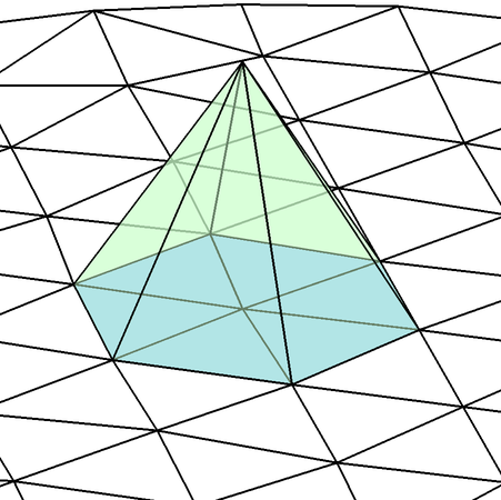
• Find a tringulation of the domain \(\Omega\) into triangular elements \(T^k\), \(k=1,\ldots,K\) and nodes \(\boldsymbol{x}_i\), \(i=1,\ldots,n\)

• Consider the space \(V_h\) of continuous functions that are linear within each element

• Use a nodal basis \(V_h=\mathrm{span}\{\varphi_1,\ldots,\varphi_n\}\) defined by \[\begin{aligned} \varphi_i\in V_h,\quad \varphi_i(\boldsymbol{x}_j)=\delta_{ij},\quad 1\le i,j\le n \end{aligned}\]

• A function \(v\in V_h\) can then be written \[\begin{aligned} v=\sum_{i=1}^n v_i\varphi_i(\boldsymbol{x}) \end{aligned}\] with the nodal interpretation \[\begin{aligned} v(\boldsymbol{x}_j)=\sum_{i=1}^n v_i\varphi_i(\boldsymbol{x}_j) = \sum_{i=1}^n v_i\delta_{ij} = v_j \end{aligned}\]

Local Basis Functions

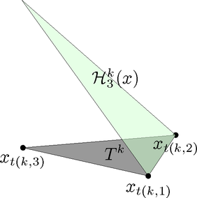
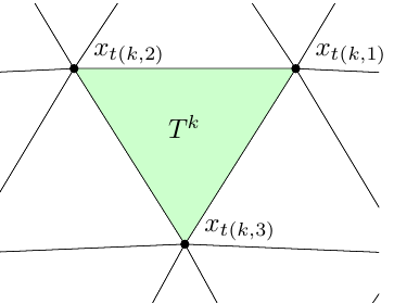
• Consider a triangular element \(T^k\) with local nodes \(\boldsymbol{x}_1^k, \boldsymbol{x}_2^k, \boldsymbol{x}_3^k\)

• The local basis functions \(\mathcal{H}_1^k,\mathcal{H}_2^k,\mathcal{H}_3^k\) are linear functions: \[\begin{aligned} \mathcal{H}_\alpha^k = c_\alpha^k + c_{x,\alpha}^k x + c_{y,\alpha}^k y,\quad \alpha=1,2,3 \end{aligned}\] with the property that \(\mathcal{H}_\alpha^k(x_\beta) = \delta_{\alpha\beta}\), \(\beta=1,2,3\)

• This leads to linear systems of equations for the coefficients: \[\begin{aligned} \begin{pmatrix} 1 & x_1^k & y_1^k \\ 1 & x_2^k & y_2^k \\ 1 & x_3^k & y_3^k \end{pmatrix} \begin{pmatrix} c_\alpha^k \\ c_{x,\alpha}^k \\ x_{y,\alpha}^k \end{pmatrix} = \begin{pmatrix} 1 \\ 0 \\ 0 \end{pmatrix} \text{ or } \begin{pmatrix} 0 \\ 1 \\ 0 \end{pmatrix} \text{ or } \begin{pmatrix} 0 \\ 0 \\ 1 \end{pmatrix} \end{aligned}\] or \(C = V^{-1}\) with coefficient matrix \(C\) and Vandermonde matrix \(V\)

Elementary Matrices and Loads

• The elementary matrix for an element \(T^k\) becomes \[\begin{aligned} A^k_{\alpha\beta} &= \int_{T^k} \frac{\partial \mathcal{H}_\alpha^k}{\partial x} \frac{\partial \mathcal{H}_\beta^k}{\partial x} + \frac{\partial \mathcal{H}_\alpha^k}{\partial y} \frac{\partial \mathcal{H}_\beta^k}{\partial y}\,dx \\ &= \mathrm{Area}^k (c_{x,\alpha}^k c_{x,\beta}^k + c_{y,\alpha}^k c_{y,\beta}^k),\quad \alpha,\beta=1,2,3 \end{aligned}\]

• The elementary load becomes \[\begin{aligned} b^k_\alpha &= \int_{T^k} f\,\mathcal{H}_\alpha^k\,dx \\ &= \text{(if $f$ constant)} \\ &= \frac{\mathrm{Area}^k}{3}f,\quad \alpha=1,2,3 \end{aligned}\]

Assembly, The Stamping Method

• Assume a local-to-global mapping \(t(k,\alpha)\), giving the global node number for local node number \(\alpha\) in element \(k\)

• The global linear system is then obtained from the elementary matrices and loads by the stamping method:
  

  \(A=0\), \(b=0\)
  for \(k=1,\ldots,K\)
  \(A(t(k,:),t(k,:)) = A(t(k,:),t(k,:)) + A^k\)
  \(b(t(k,:)) = b(t(k,:)) + b^k\)

  
   
   
  

Dirichlet Conditions

• Suppose Dirichlet conditions \(u=u_D\) are imposed on part of the boundary \(\Gamma_D\)

• Enforce \(u_{h,i} = u_D\) for all nodes \(i\) on \(\Gamma_D\) directly in the linear system of equations: \[\begin{aligned} & \qquad\qquad\qquad\,i \nonumber \\ \begin{array}{c} \\ \\ i \\ \\ \\ \end{array} &\begin{pmatrix} \\ \\ 0 & \cdots & 0 & 1 & 0 & \cdots & 0 \\ \\ \\ \end{pmatrix} u_h = \begin{pmatrix} \\ \\ u_D \\ \\ \\ \end{pmatrix} \end{aligned}\]

• Eliminate below/above diagonal of the Dirichlet nodes to retain symmetry

FEM Theory

Variational and minimization formulations

Consider the Dirichlet problem (D) \[\begin{aligned} -\nabla^2 u &= f\ \ \text{in }\Omega \\ u &= 0\ \ \text{on }\Gamma \end{aligned}\] Introduce the notation \[\begin{aligned} a(u,v) &= \int_{\Omega} \nabla u \cdot \nabla v\, dx & & \text{(bilinear form)} \\ \ell(v) &= \int_{\Omega} f v\, dx & & \text{(linear form)} \end{aligned}\] Note that \[\begin{aligned} a(u_1+u_2,v) &= a(u_1,v) + a(u_2,v) & & \text{(bilinearity)} \\ \ell(v_1+v_2) &= \ell(v_1) + \ell(v_2) & & \text{(linearity)} \\ a(u,v) &= a(v,u) & & \text{(symmetry)} \end{aligned}\] Also, \[\begin{aligned} a(u,u) &= \int_{\Omega} \|\nabla u\|^2_2\, dx \ge 0, \end{aligned}\] and if \(u=0\) on \(\Gamma\), then equality only for \(u=0\). This can then be used to define the energy norm \[\begin{aligned} \|| u \||\ \equiv \sqrt{a(u,u)} \end{aligned}\] Now, define the spaces \[\begin{aligned} L_2(\Omega) &= \{ v\ :\ v\text{ is defined on }\Omega\text{ and }\int_{\Omega} v^2\,dx <\infty\} \\ H^1(\Omega) &= \{ v\in L_2(\Omega)\ :\ \frac{\partial v}{\partial x_i}\in L_2(\Omega)\text{ for } u=1,\ldots,d \} \\ H^1_0(\Omega) &= \{v\in H^1(\Omega)\ :\ v=0\text{ on }\Gamma \} \end{aligned}\] where \(d\) is the number of space dimensions. Let \(V=H^1_0\). The solution \(u\) to (D) then satisfies a corresponding variational problem (V): \[\begin{aligned} \text{Find }u\in V\text{ s.t. } a(u,v) = \ell(v)\quad \forall v\in V \end{aligned}\] This is also called the weak form of (D), with a weak solution u. Note that a solution \(u\) of (D) is also a solution of (V), since for any \(v\in V\): \[\begin{aligned} \int_{\Omega} - \nabla^2 u v\, dx &= \int_{\Omega} f v\, dx \\ \int_{\Omega} \nabla u \cdot \nabla v\, dx - \oint_{\Gamma} \boldsymbol{n}\cdot \nabla u\, v\, ds &= \int_{\Omega} f v\, dx \\ \int_{\Omega} \nabla u \cdot \nabla v\, dx &= \int_{\Omega} f v\, dx \\ a(u,v) &= \ell(v) \end{aligned}\] where we used the fact that \(v=0\) on \(\Gamma\). The reverse can also be shown, (V) \(\Longrightarrow\) (D), if \(u\) is sufficiently regular.

Now consider the minimization problem (M): \[\begin{aligned} \text{Find }u\in V\text{ s.t. } F(u) \le F(v)\quad \forall v\in V,\quad \text{where } F(v) = \frac12 a(v,v) - \ell(v) \end{aligned}\] Suppose \(u\) solves (V). Then it also solves (M), since for any \(v\in V\), set \(w=v-u\in V\), and \[\begin{aligned} F(v) &= F(u+w) = \frac12 a(u+w,u+w) - \ell(u+w) \\ &= \frac12 a(u,u) + \frac12 a(u,w) + \frac12 a(w,v) + \frac12 a(w,w) - \ell(u) - \ell(w) \\ &= \underbrace{\frac12 a(u,u) - \ell(u)}_{F(u)} + \underbrace{a(u,w) - \ell(w)}_{=0\ \forall w\in V} + \underbrace{\frac12 a(w,w)}_{\ge 0} \ge F(u) \end{aligned}\] The reverse can also easily be shown, that is, (M) \(\Longrightarrow\) (V).

FEM formulation

Now define the FEM formulation \[\begin{aligned} \text{Find } u_h \in V_h\text{ s.t. } a(u_h,v) = \ell(v)\quad \forall v\in V_h \end{aligned}\] for some finite-dimensional subspace \(V_h\) of \(V\). Recall that the solution \(u\) to (V) satisfies \(a(u,v) = \ell(v)\) for all \(v\in V\), and in particular for all \(v\in V_h\), we have \[\begin{aligned} a(u - u_h, v) = 0 \quad \forall v\in V_h, \label{errororthogonality} \end{aligned}\] or \(a(e,v) = 0\) with the error \(e = u-u_h\). This means that the error also satisfies a corresponding minimization problem (M), with \(\ell(v) = 0\), which leads to the property: \[\begin{aligned} \frac12 a(v,v) - 0 = \frac12 \||v\||^2\text{ is minimized by }v = u-u_h = e \end{aligned}\] In other words, for any \(w_h\in V_h\), \(\||u-w_h\|| \ge \||u-u_h\||\), or the FEM formulation finds the best possible solution in the energy norm.

More generally, for any Hilbert space \(V\) with corresponding norm \(\|\cdot\|_V\), we require that

• \(a(\cdot,\cdot)\) is symmetric

• \(a(\cdot,\cdot)\) is continuous, i.e., \(\exists \gamma>0\) s.t. \(|a(v,w)| \le \gamma \|v\|_V \|w\|_V\), \(\forall v,w\in V\)

• \(a(\cdot,\cdot)\) is \(V\)-elliptic, i.e., \(\exists \alpha>0\) s.t. \(a(v,v) \ge \alpha \|v\|_V^2\), \(\forall v\in V\)

• \(\ell(\cdot)\) is continuous, i.e., \(\exists \Lambda>0\) s.t. \(|L(v)| \le \Lambda \|v\|_V\), \(\forall v\in V\)

The energy norm \(\||\cdot\||\) is then equivalent to \(\|\cdot\|_V\), that is, \(\exists c,C>0\) s.t. \[\begin{aligned} c\|v\|_V \le \||v\|| \le C \|v\|_V\quad\forall v\in V \end{aligned}\] for example with \(c=\sqrt{\alpha}\) and \(C=\sqrt{\gamma}\). This gives \[\begin{aligned} \|u-u_j\|_V \le \frac{\gamma}{\alpha} \|u-v\|_V\quad \forall v\in V_h \end{aligned}\]

Interpolants

Consider a 1-D function \(w\in V\) and its linear interpolant \(w_I\in V_h\), where \(V_h\) is a space of piecewise linear functions, defined by \(w_I(x_i) = w(x_i)\), or \[\begin{aligned} w_I(x) = \sum_{i=1}^n w(x_i) \varphi_i(x) \end{aligned}\] To find a bound on the energy norm of the difference \(w-w_I\), we first bound the derivative. Consider a single element, and note that the difference \(w-w_I\) is zero at the endpoints. A point \(x=z\) must then exists, such that \[\begin{aligned} ' = 0 \end{aligned}\] For any other point \(x\) inside the element, we then have from the fundamental theorem of calculus, \[\begin{aligned} ' = \int_z^x [w(y) - w_I(y)]''\,dy \end{aligned}\] but \(w_I(y)\) is linear, so \(w_I''(y) = 0\) and \[\begin{aligned} ' = \int_z^x w''(y)\,dy \end{aligned}\] If the element width is \(h\), this gives the bound \[\begin{aligned} \left| [w(x)-w_I(x)]' \right| \le h \max |w''| \end{aligned}\] A bound for the energy norm of \(w-w_I\) can then be derived as follows. Note that the number of elements \(T\) can be written as \(C_1/h\), for some constant \(C_1\). \[\begin{aligned} \||w-w_I\||^2 &= \sum_{k=1}^T \int_{e_k} [(w-w_I)']^2\,dx \le \frac{C_1}{h} \cdot h \cdot h^2 \cdot [\max |w''|]^2 \\ &= C_1 h^2 [\max |w''|]^2 \end{aligned}\] or \[\begin{aligned} \||w-w_I\|| \le Ch \max |w''| \end{aligned}\]

FEM error bounds

For a finite element solution \(u_h\), the optimality in the energy norm and the boundary on the interpolat leads to \[\begin{aligned} \||u-u_h\|| \le \||u-u_I\|| \le Kh\max |u''| = \mathcal{O}(h) \end{aligned}\] This implies convergence in the energy norm, at a linear rate w.r.t. the element sizes \(h\).

This result does not imply that the solution itself in, for example, the \(L_2\)-norm is quadratically convergent. However, using other techniques it can be shown that \[\begin{aligned} \|u-u_h\|_{L_2} = \mathcal{O}(h^2) \end{aligned}\] under suitable assumptions.

2-D interpolants

For piecewise interpolant on a triangular mesh in 2-D, it can be shown that \[\begin{aligned} \||w-w_I\|| &\le C h \|w\|_{H^2} \\ \|w-w_I\|_{L_2} &\le C h^2 \|w\|_{H^2} \end{aligned}\] which again leads to the energy norm bound for a finite element solution \(u_h\) \[\begin{aligned} \||u-u_h\|| \le C_1 h \|u\|_{H^2} \end{aligned}\] However, two new problems appear in 2-D:

• “Bad elements”, consider e.g. interpolation of the function \(w(x,y) = x^2\) on a triangle with corners at \((x,y)\) = \((-1,0)\), \((1,0)\), and \((0,\varepsilon)\). Since \(w(-1,0)=w(1,0)=1\), linear interpolation gives \(w_I(0,0)=1\). But \(w(0,\varepsilon)=0\), so the derivative along the \(y\)-axis: \[\begin{aligned} \frac{\partial w_I}{\partial y}(0,0) = -\frac{1}{\varepsilon} \rightarrow -\infty \text{ as } \theta \rightarrow 180^\circ \end{aligned}\] where \(\theta\) is the top angle. This does not affect the linear convergence of the energy norm as \(h\rightarrow 0\), since the worst angle \(\theta\) remains fixed, but it can cause a large constant \(C_1\) if the mesh contains bad elements.

• Lack of regularity of the solution, or geometry-induced singularities. For example on a domain with convex corners, it can be shown that \(\|u\|_{H^2}\) is not bounded which reduces the convergence rate of the FEM solution.

Some extensions

Higher order elements in 2D

For the piecewise linear case on triangular meshes, we parameterized the space of continuous functions as:

• Representing a solution \(u_i\) at the global nodes \(\boldsymbol{x}_i\)

• Using a uniquely defined linear function \(u(x,y) = a+bx+cy\) on each triangle, from the 3 corner nodes

• Continuity is enforced since the node values are single-valued, and along an edge between two elements there is a uniquely defined linear function.

This extends natually to piecewise quadratic elements:

• Introduce the edge midpoints as global nodes

• Each triangle is now associated with 6 nodes, with determines a unique quadratic function \(u(x,y)=a+bx+cy+dx^2+exy+fy^2\)

• Continuity obtained since along an edge, there is a uniquely defined quadratic

This can be generalized to Lagrange elements of any degree \(p\) in any dimension \(D\), using \(\binom{p+D}{D}\) nodes in a regular pattern.

Other PDEs

Consider the more general linear parabolic PDE: \[\begin{aligned} \rho \frac{\partial u}{\partial t} - \nabla \cdot (D\nabla u + \boldsymbol{\alpha}u) +au = f\quad \text{in }\Omega \label{generalpde} \end{aligned}\] with boundary conditions \[\begin{aligned} \boldsymbol{n}\cdot (D\nabla u+\boldsymbol{\alpha}u) &= g \qquad \text{on }\Gamma_N \\ u &= u_D \qquad \text{on }\Gamma_D \end{aligned}\] Note that the fields \(rho\), \(D\), \(\boldsymbol{\alpha}\), \(g\), and \(u_D\) in general are time and space dependent.

A standard FEM formulation for ([generalpde]) is: Find \(u_h\in V_h\) s.t. \[\begin{aligned} \int_\Omega \rho \dot{u_h} v\, dx + \int_\Omega (D\nabla u_h + \boldsymbol{\alpha}u_h)\cdot \nabla v\,dx + \int_\Omega au_h v\, dx = \int_\Omega fv\,dx + \int_{\Gamma_N} gv\,ds \end{aligned}\] for all \(v\in V_{0,h}\), where \(V_h\) is an appropriate finite dimensional space satisfying the Dirichlet conditions. Considering the all-Neumann problem, discretization with basis functions \(\varphi_i(\boldsymbol{x})\) leads to the linear system of ODEs \[\begin{aligned} M_\rho \dot{\boldsymbol{u}} + K\boldsymbol{u} + C\boldsymbol{u} + M_a \boldsymbol{u} = \boldsymbol{f} + \boldsymbol{g} \end{aligned}\] where \[\begin{aligned} M_{\rho,ij} &= \int_\Omega \rho \varphi_i \varphi_j\, dx \\ M_{a,ij} &= \int_\Omega a \varphi_i \varphi_j\, dx \\ K_{ij} &= \int_\Omega (D\nabla \varphi_j) \cdot \nabla \varphi_i\, dx \\ C_{ij} &= \int_\Omega (\boldsymbol{\alpha} \varphi_j) \cdot (\nabla \varphi_i)\, dx \\ f_i &= \int_\Omega f\varphi_i\,dx \\ g_i &= \oint_\Gamma g\varphi_i\,ds \end{aligned}\] This can be integrated in time using method of lines, with e.g. a BDF method or an implicit Runge-Kutta. Note that explicit methods can be used, but they require inversion of \(M_\rho\) and will put stability constrains on the timestep.