Implementation of Finite Element Methods
Math 228B Numerical Solutions of Differential Equations
The Poisson Problem in 2-D
Consider the problem \[\begin{aligned} -\nabla^2 u &= f \text{ in }\Omega \\ n\cdot\nabla u &= g \text{ on } \Gamma \end{aligned}\] for a domain \(\Omega\) with boundary \(\Gamma\)
Seek solution \(\hat{u}\in\hat{X}\), multiply by a test function \(v\in\hat{X}\), and integrate: \[\begin{aligned} \int_\Omega -\nabla^2 \hat{u} v\,d\Omega = \int_\Omega fv\,d\Omega \end{aligned}\]
Apply the divergence theorem and use the Neumann condition, to get the Galerkin form \[\begin{aligned} \int_\Omega \nabla \hat{u} \nabla v\,d\Omega = \int_\Omega fv\,d\Omega + \oint_\Gamma g v\,ds \end{aligned}\]
Finite Element Formulation
Expand in basis \(\hat{u}=\sum_i \hat{u}_i \phi_i(x)\), insert into the Galerkin form, and set \(v = \phi_i\), \(i=1,\ldots,n\): \[\begin{aligned} \int_\Omega \left[\sum_{j=1}^n \hat{u}_j\nabla\phi_j\right]\cdot\nabla \phi_i\,d\Omega = \int_\Omega f\phi_i\,d\Omega + \oint_\Gamma g\phi_i\,ds \end{aligned}\] Switch order of integration and summation to get the finite element formulation: \[\begin{aligned} \sum_{j=1}^n A_{ij} \hat{u}_j = b_i,\quad\text{or}\quad A\hat{u} = b \end{aligned}\] where \[\begin{aligned} A_{ij} = \int_\Omega \nabla\phi_i\cdot\nabla\phi_j\,d\Omega, \quad b_i = \int_\Omega f \phi_i + \oint_\Gamma g\phi_i\,ds \end{aligned}\]
Discretization
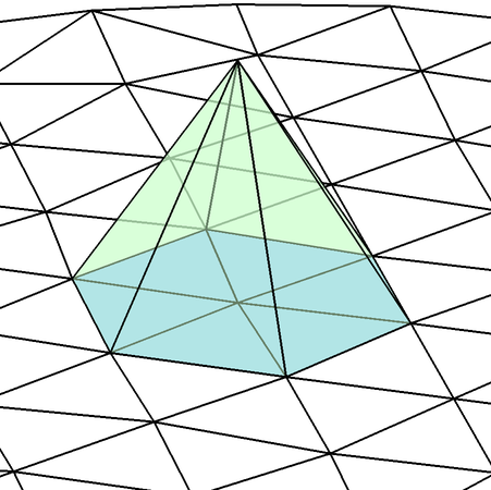
Find a tringulation of the domain \(\Omega\) into triangular elements \(T^k\), \(k=1,\ldots,K\) and nodes \(x_i\), \(i=1,\ldots,n\)
Consider the space \(\hat{X}\) of continuous functions that are linear within each element
Use a nodal basis \(\hat{X}=\mathrm{span}\{\phi_1,\ldots,\phi_n\}\) defined by \[\begin{aligned} \phi_i\in \hat{X},\quad \phi_i(x_j)=\delta_{ij},\quad 1\le i,j\le n \end{aligned}\]
A function \(v\in\hat{X}\) can then be written \[\begin{aligned} v=\sum_{i=1}^n v_i\phi_i(x) \end{aligned}\] with the nodal interpretation \[\begin{aligned} v(x_j)=\sum_{i=1}^n v_i\phi_i(x) = \sum_{i=1}^n v_i\delta_{ij} = v_j \end{aligned}\]
Local Basis Functions
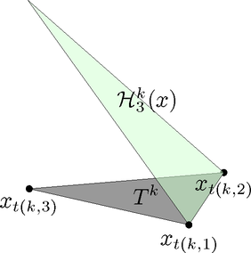
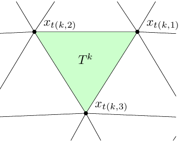
Consider a triangular element \(T^k\) with local nodes \(x_1^k, x_2^k, x_3^k\)
The local basis functions \(\mathcal{H}_1^k,\mathcal{H}_2^k,\mathcal{H}_3^k\) are linear functions: \[\begin{aligned} \mathcal{H}_\alpha^k = c_\alpha^k + c_{x,\alpha}^k x + c_{y,\alpha}^k y,\quad \alpha=1,2,3 \end{aligned}\] with the property that \(\mathcal{H}_\alpha^k(x_\beta) = \delta_{\alpha\beta}\), \(\beta=1,2,3\)
This leads to linear systems of equations for the coefficients: \[\begin{aligned} \begin{pmatrix} 1 & x_1^k & y_1^k \\ 1 & x_2^k & y_2^k \\ 1 & x_3^k & y_3^k \end{pmatrix} \begin{pmatrix} c_\alpha^k \\ c_{x,\alpha}^k \\ x_{y,\alpha}^k \end{pmatrix} = \begin{pmatrix} 1 \\ 0 \\ 0 \end{pmatrix} \text{ or } \begin{pmatrix} 0 \\ 1 \\ 0 \end{pmatrix} \text{ or } \begin{pmatrix} 0 \\ 0 \\ 1 \end{pmatrix} \end{aligned}\] or \(C = V^{-1}\) with coefficient matrix \(C\) and Vandermonde matrix \(V\)
Elementary Matrices and Loads
The elementary matrix for an element \(T^k\) becomes \[\begin{aligned} A^k_{\alpha\beta} &= \int_{T^k} \frac{\partial \mathcal{H}_\alpha^k}{\partial x} \frac{\partial \mathcal{H}_\beta^k}{\partial x} + \frac{\partial \mathcal{H}_\alpha^k}{\partial y} \frac{\partial \mathcal{H}_\beta^k}{\partial y}\,d\Omega \\ &= \mathrm{Area}^k (c_{x,\alpha}^k c_{x,\beta}^k + c_{y,\alpha}^k c_{y,\beta}^k),\quad \alpha,\beta=1,2,3 \end{aligned}\]
The elementary load becomes \[\begin{aligned} b^k_\alpha &= \int_{T^k} f\,\mathcal{H}_\alpha^k\,d\Omega \\ &= \text{(if $f$ constant)} \\ &= \frac{\mathrm{Area}^k}{3}f,\quad \alpha=1,2,3 \end{aligned}\]
Assembly, The Stamping Method
Assume a local-to-global mapping \(t(k,\alpha)\), giving the global node number for local node number \(\alpha\) in element \(k\)
The global linear system is then obtained from the elementary matrices and loads by the stamping method:
\(A=0\), \(b=0\) for \(k=1,\ldots,K\) \(A(t(k,:),t(k,:)) = A(t(k,:),t(k,:)) + A^k\) \(b(t(k,:)) = b(t(k,:)) + b^k\)
Dirichlet Conditions
Suppose Dirichlet conditions \(u=u_D\) are imposed on part of the boundary \(\Gamma_D\)
Enforce \(\hat{u}_i = u_D\) for all nodes \(i\) on \(\Gamma_D\) directly in the linear system of equations: \[\begin{aligned} & \qquad\qquad\qquad\,i \\ \begin{array}{c} \\ \\ i \\ \\ \\ \end{array} &\begin{pmatrix} \\ \\ 0 & \cdots & 0 & 1 & 0 & \cdots & 0 \\ \\ \\ \end{pmatrix} \hat{u} = \begin{pmatrix} \\ \\ u_D \\ \\ \\ \end{pmatrix} \end{aligned}\]