Finite Difference Methods for PDEs
Math 228B Numerical Solutions of Differential Equations
Finite Difference Approximations
Finite Difference Approximations
\[\begin{aligned} D_+ u(\bar{x}) &= \frac{u(\bar{x}+h)-u(\bar{x})}{h} = u'(\bar{x})+\frac{h}{2} u''(\bar{x}) + \mathcal{O}(h^2) \\ D_- u(\bar{x}) &= \frac{u(\bar{x})-u(\bar{x}-h)}{h} = u'(\bar{x})-\frac{h}{2} u''(\bar{x}) + \mathcal{O}(h^2) \\ D_0 u(\bar{x}) &= \frac{u(\bar{x}+h)-u(\bar{x}-h)}{2h} = u'(\bar{x})+\frac{h^2}{6} u'''(\bar{x}) + \mathcal{O}(h^4) \\ D^2 u(\bar{x}) &= \frac{u(\bar{x}-h)-2u(\bar{x})+u(\bar{x}+h)}{h^2} \\ &= u''(\bar{x}) + \frac{h^2}{12}u''''(\bar{x})+\mathcal{O}(h^4) \end{aligned}\]
Method of Undetermined Coefficients
Find approximation to \(u^{(k)}(\bar{x})\) based on \(u(x)\) at \(x_1,x_2,\ldots,x_n\)
Write \(u(x_i)\) as Taylor series centered at \(\bar{x}\): \[\begin{aligned} u(x_i) &= u(\bar{x}) + (x_i-\bar{x})u'(\bar{x}) + \cdots + \frac{1}{k!} (x_i-\bar{x})^k u^{(k)}(\bar{x}) + \cdots \end{aligned}\]
Seek approximation of the form \[\begin{aligned} u^{(k)}(\bar{x}) = c_1 u(x_1) + c_2 u(x_2) + \cdots + c_n u(x_n) + \mathcal{O}(h^p) \end{aligned}\]
Collect terms multiplying \(u(\bar{x})\), \(u'(\bar{x})\), etc, to obtain: \[\begin{aligned} \frac{1}{(i-1)!} \sum_{j=1}^n c_j (x_j-\bar{x})^{(i-1)} = \begin{cases} 1 & \text{if } i-1=k \\ 0 & \text{otherwise.} \end{cases} \end{aligned}\]
Nonsingular Vandermonde system if \(x_j\) are distinct
Finite difference stencils, Julia implementation
"""
    c = mkfdstencil(x, xbar, k)

Compute the coefficients `c` in a finite difference approximation of a function
defined at the grid points `x`, evaluated at `xbar`, of order `k`.
"""
function mkfdstencil(x, xbar, k)
    n = length(x)
    A = @. (x[:]' - xbar) ^ (0:n-1) / factorial(0:n-1)
    b = (1:n) .== k+1
    c = A \ b
end
Examples:
julia> println(mkfdstencil([-1 0 1], 0, 2)) # Centered 2nd derivative
[1.0, -2.0, 1.0]

julia> println(mkfdstencil([0 1 2], 0, 1))  # One-sided (right) 1st derivative
[-1.5, 2.0, -0.5]

julia> println(mkfdstencil(-2:2, 0//1, 2))  # 4th order 5-point stencil, rational
Rational{Int64}[-1//12, 4//3, -5//2, 4//3, -1//12]
Boundary Value Problems
The Finite Difference Method
Consider the Poisson equation with Dirichlet conditions: \[\begin{aligned} u''(x) = f(x),\quad 0<x<1,\quad u(0)=\alpha,\quad u(1)=\beta \end{aligned}\]
Introduce \(n\) uniformly spaced grid points \(x_j=jh\), \(h=1/(n+1)\)
Set \(u_0=\alpha\), \(u_{n+1}=\beta\), and use the three-point difference approximation to get the discretization \[\begin{aligned} \frac{1}{h^2} (u_{j-1} - 2u_j + u_{j+1}) = f(x_j),\quad j=1,\ldots,n \end{aligned}\]
This can be written as a linear system \(Au=f\) with
\[\begin{aligned} A=\frac{1}{h^2} \begin{bmatrix} -2 & 1 & & \\ 1 & -2 & 1 & \\ & & \ddots & \\ & & 1 & -2 \end{bmatrix} \quad u= \begin{bmatrix} u_1 \\ u_2 \\ \vdots \\ u_n \end{bmatrix} \quad f= \begin{bmatrix} f(x_1) - \alpha/h^2 \\ f(x_2) \\ \vdots \\ f(x_n)-\beta/h^2 \end{bmatrix} \end{aligned}\]
Errors and Grid Function Norms
The error \(e=u-\hat{u}\) where \(u\) is the numerical solution and \(\hat{u}\) is the exact solution \[\begin{aligned} \hat{u} = \begin{bmatrix} u(x_1) \\ \vdots \\ u(x_n) \end{bmatrix} \end{aligned}\]
Measure errors in grid function norms, which are approximations of integrals and scale correctly as \(n\rightarrow\infty\) \[\begin{aligned} \|e\|_\infty &= \max_j |e_j| \\ \|e\|_1 &= h \sum_j |e_j| \\ \|e\|_2 &= \left( h\sum_j |e_j|^2 \right)^{1/2} \end{aligned}\]
Local Truncation Error
Insert the exact solution \(u(x)\) into the difference scheme to get the local truncation error: \[\begin{aligned} \tau_j &= \frac{1}{h^2} (u(x_{j-1}) - 2u(x_j) + u(x_{j+1})) - f(x_j) \\ &= u''(x_j) + \frac{h^2}{12} u''''(x_j) + \mathcal{O}(h^4) - f(x_j) \\ &= \frac{h^2}{12} u''''(x_j) + \mathcal{O}(h^4) \end{aligned}\] or \[\begin{aligned} \tau=\begin{bmatrix} \tau_1 \\ \vdots \\ \tau_n \end{bmatrix} = A\hat{u}-f \end{aligned}\]
Errors
Linear system gives error in terms of LTE: \[\begin{aligned} \left\{ \begin{array}{ll} Au = f \\ A\hat{u} = f+\tau \end{array} \right. \Longrightarrow Ae = -\tau \end{aligned}\]
Introduce superscript \(h\) to indicate that a problem depends on the grid spacing, and bound the norm of the error: \[\begin{aligned} A^h e^h &= -\tau^h \\ e^h &= - (A^h)^{-1} \tau^h \\ \|e^h\| &= \|(A^h)^{-1}\tau^h\| \le \|(A^h)^{-1}\|\cdot\|\tau^h\| \end{aligned}\]
If \(\|(A^h)^{-1}\|\le C\) for \(h\le h_0\), then \[\begin{aligned} \|e^h\|\le C \cdot \|\tau^h\| \rightarrow 0 \text{ if } \|\tau^h\|\rightarrow 0\text{ as }h\rightarrow 0 \end{aligned}\]
Stability, Consistency, and Convergence
A method \(A^hu^h=f^h\) is stable if \((A^h)^{-1}\) exists and \(\|(A^h)^{-1}\|\le C\) for \(h\le h_0\)
It is consistent with the DE if \(\|\tau^h\|\rightarrow 0\) as \(h\rightarrow 0\)
It is convergent if \(\|e^h\|\rightarrow 0\) as \(h\rightarrow 0\)
Consistency + Stability \(\Longrightarrow\) Convergence
since \(\|e^h\|\le \|(A^h)^{-1}\|\cdot\|\tau^h\| \le C\cdot \|\tau^h\| \rightarrow 0\). A stronger statement is
\(\mathcal{O}(h^p)\) LTE + Stability \(\Longrightarrow\) \(\mathcal{O}(h^p)\) global error
Stability in the 2-Norm
In the 2-norm, we have \[\begin{aligned} \|A\|_2 &= \rho(A) = \max_p |\lambda_p| \\ \|A^{-1}\|_2 &= \frac{1}{\min_p |\lambda_p|} \end{aligned}\]
For our model problem matrix, we have explicit expressions for the eigenvectors/eigenvalues:
\[\begin{aligned} A=\frac{1}{h^2} \begin{bmatrix} -2 & 1 & & \\ 1 & -2 & 1 & \\ & & \ddots & \\ & & 1 & -2 \end{bmatrix} \end{aligned}\]
\[\begin{aligned} u_j^p &= \sin (p\pi j h) \\ \lambda_p &= \frac{2}{h^2}(\cos(p\pi h)-1) \end{aligned}\]
The smallest eigenvalue is \[\begin{aligned} \lambda_1 = \frac{2}{h^2}(\cos(\pi h)-1) = -\pi^2 +\mathcal{O}(h^2) \Longrightarrow \text{ Stability} \end{aligned}\]
Convergence in the 2-Norm
This gives a bound on the error \[\begin{aligned} \|e^h\|_2 \le \|(A^h)^{-1}\|_2\cdot\|\tau^h\|_2 \approx \frac{1}{\pi^2}\|\tau^h\|_2 \end{aligned}\]
Since \(\tau_j^h\approx \frac{h^2}{12} u''''(x_j)\), \[\begin{aligned} \|\tau^h\|_2 \approx \frac{h^2}{12} \|u''''\|_2 = \frac{h^2}{12}\|f''\|_2 \Longrightarrow \|e^h\|_2 = \mathcal{O}(h^2) \end{aligned}\]
While this implies convergence in the max-norm, 1/2 order is lost because of the grid function norm: \[\begin{aligned} \|e^h\|_\infty \le \frac{1}{\sqrt{h}} \|e^h\|_2 = \mathcal{O}(h^{3/2}) \end{aligned}\]
But it can be shown that \(\|(A^h)^{-1}\|_\infty=\mathcal{O}(1)\), which implies \(\|e^h\|_\infty = \mathcal{O}(h^2)\)
Neumann Boundary Conditions
Consider the Poisson equation with Neumann/Dirichlet conditions: \[\begin{aligned} u''(x) = f(x),\quad 0<x<1,\quad u'(0)=\sigma,\quad u(1)=\beta \end{aligned}\]
Second-order accurate one-sided difference approximation: \[\begin{aligned} \frac{1}{h}\left(-\frac32 u_0 + 2u_1 - \frac12 u_2\right) = \sigma \end{aligned}\] \[\begin{aligned} \frac{1}{h^2} \begin{bmatrix} -\frac{3h}{2} & 2h & -\frac{h}{2} & & \\ 1 & -2 & 1 & &\\ & & \ddots & &\\ & & 1 & -2 & 1 \\ & & & 0 & h^2 \end{bmatrix} \begin{bmatrix} u_0 \\ u_1 \\ \vdots \\ u_n \\ u_{n+1} \end{bmatrix} = \begin{bmatrix} \sigma \\ f(x_1) \\ \vdots \\ f(x_n) \\ \beta \end{bmatrix} \end{aligned}\] Most general approach.
Finite Difference Methods for Elliptic Problems
Elliptic Partial Differential Equations
Consider the elliptic PDE below, the Poisson equation: \[\begin{aligned} \nabla^2 u(x,y) \equiv \frac{\partial ^2 u}{\partial x^2} (x,y) + \frac{\partial ^2 u}{\partial y^2} (x,y) = f(x,y) \end{aligned}\] on the rectangular domain \[\begin{aligned} \Omega = \{ (x,y)\ |\ a<x<b, c<y<d \} \end{aligned}\] with Dirichlet boundary conditions \(u(x,y) = g(x,y)\) on the boundary \(\Gamma=\partial \Omega\) of \(\Omega\).
Introduce a two-dimensional grid by choosing integers \(n,m\) and defining step sizes \(h=(b-a)/n\) and \(k = (d-c)/m\). This gives the point coordinates (mesh points): \[\begin{aligned} x_i &= a+ih,\qquad i=0,1,\ldots,n \\ y_i &= c+jk,\qquad j=0,1,\ldots,m \end{aligned}\]
Finite Difference Discretization
Discretize each of the second derivatives using finite differences on the grid: \[\begin{aligned} &\frac{u(x_{i+1},y_j) - 2u(x_i,y_j) + u(x_{i-1},y_j)}{h^2} + \\ &\frac{u(x_{i},y_{j+1}) - 2u(x_i,y_j) + u(x_{i},y_{j-1})}{k^2} \\ & \quad = f(x_i,y_j) + \frac{h^2}{12} \frac{\partial^4 u}{\partial x^4}(x_i,y_j) + \frac{k^2}{12} \frac{\partial^4 u}{\partial y^4} (x_i,y_j) + \mathcal{O}(h^4 + k^4) \end{aligned}\] for \(i=1,2,\ldots,n-1\) and \(j=1,2,\ldots,m-1\), with boundary conditions \[\begin{aligned} u(x_0,y_j) &= g(x_0,y_j),\quad u(x_n,y_j)=g(x_n,y_j),\quad j=0,\ldots,m \\ u(x_i,y_0) &= g(x_i,y_0),\quad u(x_i,y_0)=g(x_i,y_m),\quad i=1,\ldots,n-1 \end{aligned}\]
Finite Difference Discretization
The corresponding finite-difference method for \(u_{i,j} \approx u(x_i,y_i)\) is \[\begin{aligned} &2\left[ \left(\frac{h}{k}\right)^2 + 1 \right] u_{ij} -(u_{i+1,j} + u_{i-1,j}) - \\ & \qquad \left(\frac{h}{k}\right)^2(u_{i,j+1} + u_{i,j-1}) = -h^2 f(x_i,y_j) \end{aligned}\] for \(i=1,2,\ldots,n-1\) and \(j=1,2,\ldots,m-1\), with boundary conditions \[\begin{aligned} u_{0j} &= g(x_0,y_j),\quad u_{nj}=g(x_n,y_j),\quad j=0,\ldots,m \\ u_{i0} &= g(x_i,y_0),\quad u_{im}=g(x_i,y_m),\quad i=1,\ldots,n-1 \end{aligned}\] Define \(f_{ij} = f(x_i,y_i)\) and suppose \(h=k\), to get the simple form \[\begin{aligned} u_{i+1,j} + u_{i-1,j} + u_{i,j+1} + u_{i,j-1} - 4 u_{i,j} = h^2 f_{ij} \end{aligned}\]
FDM for Poisson, Julia implementation
Convergence in the 2-Norm
For the homogeneous Dirichlet problem on the unit square, convergence in the 2-norm is shown in exactly the same way as for the corresponding BVP
Taylor expansions show that \[\begin{aligned} \tau_{ij} = \frac{1}{12} h^2 (u_{xxxx} + u_{yyyy}) + \mathcal{O}(h^4) \end{aligned}\]
It can be shown that the smallest eigenvalue of \(A^h\) is \(-2\pi^2 + \mathcal{O}(h^2)\), and the spectral radius of \((A^h)^{-1}\) is approximately \(1/2\pi^2\)
As before, this gives \(\|e^h\|_2 = \mathcal{O}(h^2)\)
Non-Rectangular Domains
Poisson in 2D non-rectangular domain
Consider the Poisson problem on the non-rectangular domain \(\Omega\) with boundary \(\Gamma = \Gamma_D \cup \Gamma_N = \partial \Omega\): \[\begin{aligned} -\nabla^2 u &= f & & \text{in }\Omega\\ u &= g & & \text{on }\Gamma_D \\ \frac{\partial u}{\partial n} &= r & & \text{on }\Gamma_N \end{aligned}\]
Consider a mapping between a rectangular reference domain \(\hat{\Omega}\) and the actual physical domain \(\Omega\)
Find an equivalent problem that can be solved in \(\hat{\Omega}\)

Poisson in 2D non-rectangular domainTransformed derivatives
Use the chain rule to transform the derivatives of \(u\) in the physical domain: \[\begin{aligned} u(x,y) = u(x(\xi,\eta), y(\xi,\eta))\quad\Longrightarrow\quad \begin{aligned} u_x &= \xi_x u_\xi+ \eta_x u_\eta \\ u_y &= \xi_y u_\xi+ \eta_y u_\eta \end{aligned} \end{aligned}\]
Determine the terms \(\xi_x,\eta_x,\xi_y,\eta_y\) by the mapped derivatives:
\[\begin{aligned} \xi = \xi(x,y) \\ \eta = \eta(x,y) \end{aligned}\] \[\begin{aligned} \begin{pmatrix} d\xi \\ d\eta \end{pmatrix} = \begin{pmatrix} \xi_x & \xi_y \\ \eta_x & \eta_y \end{pmatrix} \begin{pmatrix} dx \\ dy \end{pmatrix} \end{aligned}\]
\[\begin{aligned} x = x(\xi, \eta) \\ y = y(\xi, \eta) \end{aligned}\] \[\begin{aligned} \begin{pmatrix} dx \\ dy \end{pmatrix} = \begin{pmatrix} x_\xi & x_\eta \\ y_\xi & y_\eta \end{pmatrix} \begin{pmatrix} d\xi \\ d\eta \end{pmatrix} \end{aligned}\]
\[\begin{aligned} \Longrightarrow \begin{pmatrix} \xi_x & \xi_y \\ \eta_x & \eta_y \end{pmatrix} = \begin{pmatrix} x_\xi & x_\eta \\ y_\xi & y_\eta \end{pmatrix}^{-1} = \frac{1}{J} \begin{pmatrix} y_\eta & -x_\eta \\ -y_\xi & x_\xi \end{pmatrix} \end{aligned}\]
where \(J=x_\xi y_\eta - x_\eta y_\xi\)
Poisson in 2D non-rectangular domainTransformed equations
Using the derivative expressions, we can transform all the derivatives and the equation \(-(u_{xx} + u_{yy}) = f\) becomes \[\begin{aligned} -\frac{1}{J^2} (a u_{\xi\xi} -2bu_{\xi\eta} +c u_{\eta\eta} +d u_{\eta} + e u_{\xi}) = f \end{aligned}\] where \[\begin{aligned} a &= x^2_\eta + y^2_\eta & b &= x_\xi x_\eta + y_\xi y_\eta & c &=x^2_\xi + y^2_\xi \\ d &= \frac{y_\xi\alpha - x_\xi \beta}{J} & e &= \frac{x_\eta\beta - y_\eta \alpha}{J} \end{aligned}\] with \[\begin{aligned} \alpha &= a x_{\xi\xi} -2b x_{\xi\eta} + c x_{\eta\eta} \\ \beta &= a y_{\xi\xi} -2b y_{\xi\eta} + c y_{\eta\eta} \end{aligned}\]
Poisson in 2D non-rectangular domainNormal derivatives
The normal \(\boldsymbol{n}\) in the physical domain is in the direction of
\(\nabla\eta\) or \(\nabla\xi\).For example, on the top boundary \(\eta=1\) we have \[\begin{aligned} \boldsymbol{n} = (n^x, n^y) = \frac{1}{\sqrt{\eta^2_x + \eta^2_y}} (\eta_x, \eta_y) = \frac{1}{\sqrt{x^2_\xi + y^2_\xi}} (-y_\xi, x_\xi) \end{aligned}\]
This gives the normal derivative \[\begin{aligned} \hspace{-5mm} \frac{\partial u}{\partial n} = u_x n^x + u_y n^y = \frac{1}{J} \left[ (y_\eta n^x - x_\eta n^y) u_\xi + (-y_\xi n^x + x_\xi n^y) u_\eta \right] \end{aligned}\]
Finite Difference Methods for Parabolic Problems
Parabolic equations
Model problem: The heat equation: \[\begin{aligned} \frac{\partial u}{\partial t} - \nabla \cdot (\kappa \nabla u) = f \end{aligned}\] where
\(u=u(\boldsymbol{x},t)\) is the temperature at a given point and time
\(\kappa\) is the heat capacity (possibly \(\boldsymbol{x}\)- and \(t\)-dependent)
\(f\) is the source term (possibly \(\boldsymbol{x}\)- and \(t\)-dependent)
Need initial conditions at some time \(t_0\): \[\begin{aligned} u(\boldsymbol{x},t_0) = \eta(\boldsymbol{x}) \end{aligned}\]
Need boundary conditions at domain boundary \(\Gamma\):
Dirichlet condition (prescribed temperature): \(u = u_D\)
Neumann condition (prescribed heat flux): \(\boldsymbol{n}\cdot(\kappa \nabla u) = g_N\)
1D discretization
Initial case: One space dimension, \(\kappa=1\), \(f=0\): \[\begin{aligned} u_t = \kappa u_{xx}, \qquad 0\le x \le 1 \end{aligned}\] with boundary conditions \(u(0,t)=g_0(t)\), \(u(1,t)=g_1(t)\)
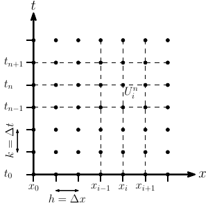
Introduce finite difference grid: \[\begin{aligned} x_i = ih,\quad t_n = nk \end{aligned}\] with mesh spacing \(h=\Delta x\) and time step \(k=\Delta t\).
Approximate the solution \(u\) at grid point \((x_i,t_n\)): \[\begin{aligned} U_i^n \approx u(x_i, t_n) \end{aligned}\]
Numerical schemes: FTCS
FTCS (Forward in time, centered in space): \[\begin{aligned} \frac{U_i^{n+1} - U_i^n}{k} = \frac{1}{h^2} \left( U_{i-1}^n - 2U_i^n + U_{i+1}^n \right) \end{aligned}\] or, as an explicit expression for \(U_i^{n+1}\), \[\begin{aligned} U_i^{n+1} = U_i^n + \frac{k}{h^2} \left( U_{i-1}^n - 2U_i^n + U_{i+1}^n \right) \end{aligned}\]
Explicit one-step method in time
Boundary conditions naturally implemented by setting \[\begin{aligned} U_0^n = g_0(t_n),\qquad U_{m+1}^n = g_1(t_n) \end{aligned}\]
FTCS, Julia implementation
using PyPlot, LinearAlgebra, DifferentialEquations
"""
Solves the 1D heat equation with the FTCS scheme (Forward-Time,
Centered-Space), using grid size `m` and timestep multiplier `kmul`.
Integrates until final time `T` and plots each solution.
"""
function heateqn_ftcs(m=100; T=0.2, kmul=0.5)
    # Discretization
    h = 1.0 / (m+1)
    x = h * (0:m+1)
    k = kmul*h^2
    N = ceil(Int, T/k)

    u = exp.(-(x .- 0.25).^2 / 0.1^2) .+ 0.1sin.(10*2π*x)  # Initial conditions
    u[[1,end]] .= 0  # Dirichlet boundary conditions u(0) = u(1) = 0

    clf(); axis([0, 1, -0.1, 1.1]); grid(true); ph, = plot(x,u) # Setup plotting
    for n = 1:N
        u[2:m+1] += k/h^2 * (u[1:m] .- 2u[2:m+1] + u[3:m+2])
        if mod(n, 10) == 0  # Plot every 10th timestep
            ph[:set_data](x,u), pause(1e-3)
        end
    end
end
Numerical schemes: Crank-Nicolson
Crank-Nicolson – like FTCS, but use average of space derivative at time steps \(n\) and \(n+1\): \[\begin{aligned} \hspace{-5mm} \frac{U_i^{n+1} - U_i^n}{k} &= \frac12 \left( D^2 U_i^n + D^2 U_i^{n+1} \right) \\ &= \frac{1}{2h^2} \left( U_{i-1}^n - 2U_i^n + U_{i+1}^n + U_{i-1}^{n+1} - 2U_i^{n+1} + U_{i+1}^{n+1} \right) \end{aligned}\] or \[\begin{aligned} \hspace{-5mm} -rU_{i-1}^{n+1} + (1+2r) U_i^{n+1} -rU_{i+1}^{n+1} = rU_{i-1}^n + (1-2r) U_i^n +rU_{i+1}^n \end{aligned}\] where \(r=k/2h^2\)
Implicit one-step method in time \(\Longrightarrow\) need to solve tridiagonal system of equations
Crank-Nicolson, Julia implementation
"""
Solves the 1D heat equation with the Crank−Nicolson scheme,
using grid size `m` and timestep multiplier `kmul`.
Integrates until final time `T` and plots each solution.
"""
function heateqn_cn(m=100; T=0.2, kmul=50)
    # Discretization
    h = 1.0 / (m+1)
    x = h * (0:m+1)
    k = kmul*h^2
    N = ceil(Int, T/k)

    u = exp.(-(x .- 0.25).^2 / 0.1^2) .+ 0.1sin.(10*2π*x)  # Initial conditions
    u[[1,end]] .= 0  # Dirichlet boundary conditions u(0) = u(1) = 0

    # Form the matrices in the Crank-Nicolson scheme (Left and right)
    A = SymTridiagonal(-2ones(m), ones(m-1)) / h^2
    LH = I - A*k/2
    RH = I + A*k/2

    clf(); axis([0, 1, -0.1, 1.1]); grid(true); ph, = plot(x,u) # Setup plotting
    for n = 1:N
        u[2:m+1] = LH \ (RH * u[2:m+1])  # Note ()'s for efficient evaluation
        ph[:set_data](x,u), pause(1e-3)  # Plot every timestep
    end
end
Local truncation error
LTE: Insert exact solution \(u(x,t)\) into difference equations
Ex: FTCS \[\begin{aligned} \hspace{-12mm} \tau(x,t) = \frac{u(x,t+k)-u(x,t)}{k} - \frac{1}{h^2}(u(x-h,t)-2u(x,t)+u(x+h,t)) \end{aligned}\] Assume \(u\) smooth enough and expand in Taylor series: \[\begin{aligned} \hspace{-10mm} \tau(x,t) = \left(u_t + \frac12 k u_{tt} + \frac16 k^2 u_{ttt} + \cdots \right) - \left( u_{xx} + \frac{1}{12} h^2 u_{xxxx} + \cdots \right) \end{aligned}\] Use the equation: \(u_t=u_{xx}\), \(u_{tt} = u_{txx} = u_{xxxx}\): \[\begin{aligned} \tau(x,t) = \left( \frac12 k - \frac{1}{12} h^2 \right) u_{xxxx} + O(k^2 + h^4) = O(k+h^2) \end{aligned}\] First order accurate in time, second order accurate in space
Ex: For Crank-Nicolson, \(\tau(x,t) = O(k^2+h^2)\)
Consistent method if \(\tau(x,t)\rightarrow 0\) as \(k,h\rightarrow 0\)
Method of Lines
Discretize PDE in space, integrate resulting semidiscrete system of ODEs using standard schemes
Ex: Centered in space \[\begin{aligned} U'_i(t) = \frac{1}{h^2} (U_{i-1}(t) - 2U_i(t) + U_{i+1}(t)),\quad i=1,\ldots,m \end{aligned}\] or in matrix form: \(U'(t) = AU(t) + g(t)\), where
\[\begin{aligned} A = \frac{1}{h^2} \begin{bmatrix} -2 & 1 & & & & \\ 1 & -2 & 1 & & & \\ & 1 & -2 & 1 & & \\ & & \ddots & \ddots & \ddots & \\ & & & 1 & -2 & 1 \\ & & & & 1 & -2 \end{bmatrix},\quad g(t) = \frac{1}{h^2} \begin{bmatrix} g_0(t) \\ 0 \\ 0 \\ \vdots \\ 0 \\ g_1(t) \end{bmatrix} \end{aligned}\]
Solve the centered semidiscrete system using:
Forward Euler \(U^{n+1} = U^n + kf(U^n)\)
\(\qquad \Longrightarrow\) the FTCS methodTrapezoidal method \(U^{n+1} = U^n + \frac{k}{2}(f(U^n)+f(U^{n+1}))\)
\(\qquad \Longrightarrow\) the Crank-Nicolson method
Heat equation, method of lines using black-box ODE solver
"""
Solves the 1D heat equation using Method of Lines with ODE solvers from
DifferentialEquations.jl. Grid size `m`, integrates until final time `T`
and plots a total of `nsteps` solutions.
"""
function heateqn_odesolver(m=100; T=0.2, nsteps=100)
    # Discretization
    h = 1.0 / (m+1)
    x = h * (0:m+1)

    u = exp.(-(x .- 0.25).^2 / 0.1^2) .+ 0.1sin.(10*2π*x)  # Initial conditions
    u[[1,end]] .= 0  # Dirichlet boundary conditions u(0) = u(1) = 0

    fode(u,p,t) = ([0; u[1:m+1]] .- 2u .+ [u[2:m+2]; 0]) / h^2 # RHS du/dt = f(u)
    prob = ODEProblem(fode, u, (0,T))
    sol = solve(prob, alg_hints=[:stiff], saveat=T / nsteps)

    # Animate solution
    clf(); axis([0, 1, -0.1, 1.1]); grid(true); ph, = plot(x,u)  # Setup plotting
    for n = 1:length(sol)
        ph[:set_data](x,sol.u[n]), pause(1e-3) # Update plot
    end
end
Method of Lines, Stability
Stability requires \(k\lambda\) to be inside the absolute stability region, for all eigenvalues \(\lambda\) of \(A\)
For the centered differences, the eigenvalues are
\[\begin{aligned} \lambda_p = \frac{2}{h^2} (\cos(p\pi h) - 1),\quad p=1,\ldots,m \end{aligned}\]
or, in particular, \(\lambda_m\approx -4/h^2\)
Euler gives \(-2\le -4k/h^2 \le 0\), or \[\begin{aligned} \frac{k}{h^2}\le \frac12 \end{aligned}\] \(\Longrightarrow\) time step restriction for FTCS
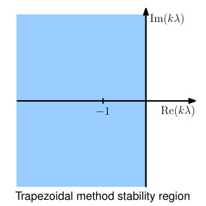
Trapezoidal method A-stable \(\Longrightarrow\) Crank-Nicolson is stable for any time step \(k>0\)
Convergence
For convergence, \(k\) and \(h\) must in general approach zero at appropriate rates, for example \(k\rightarrow 0\) and \(k/h^2 \le 1/2\)
Write the methods as \[\begin{aligned} U^{n+1} = B(k) U^n + b^n(k) \ \ (*) \end{aligned}\] where, e.g., \(B(k) = I+kA\) for forward Euler and \(B(k) = \left( I-\frac{k}{2} A \right)^{-1} \left( I+\frac{k}{2} A \right)\) for Crank-Nicolson
A linear method of the form (*) is Lax-Richtmyer stable if,
for each time \(T\), these is a
constant \(C_T>0\) such that \[\begin{aligned}
\| B(k)^n \| \le C_T
\end{aligned}\]
for all \(k>0\) and integers \(n\) for which \(kn\le T\).
A consistent linear method of the form (*) is convergent if and only if it is Lax-Richtmyer stable.
Lax Equivalence Theorem
Proof. Consider the numerical scheme applied to the
numerical solution \(U\) and the exact
solution \(u(x,t)\): \[\begin{aligned}
U^{n+1} &= BU^n + b^n \\
u^{n+1} &= Bu^n + b^n + k\tau^n
\end{aligned}\]
Subtract to get difference equation for the error \(E^n = U^n - u^n\): \[\begin{aligned}
E^{n+1} = BE^n - k\tau^n, \quad\text{or}\quad
E^N = B^NE^0 - k\sum_{n=1}^N B^{N-n}\tau^{n-1}
\end{aligned}\]
Bound the norm, use Lax-Richtmyer stability and \(Nk\le T\): \[\begin{aligned}
\|E^N\| &\le \|B^N\| \|E^0\| + k
\sum_{n=1}^N \|B^{N-n}\| \|\tau^{n-1}\| \\
& \le C_T \| E^0 \| + T C_T \max_{1\le n\le N} \|\tau^{n-1} \|
\rightarrow 0
\text{ as } k\rightarrow 0
\end{aligned}\]
provided \(\|\tau\|\rightarrow 0\) and
that the initial data \(\|E^0\|\rightarrow
0\). ◻
Convergence
For the FTCS method, \(B(k) = I+kA\) is symmetric, so \(\|B(k)\|_2 = \rho(B) \le 1\) if \(k\le h^2/2\). Therefore, it is Lax-Richtmyer stable and convergent, under this restriction.
For the Crank-Nicolson method, \(B(k) = \left( I-\frac{k}{2} A \right)^{-1} \left( I+\frac{k}{2} A \right)\) is symmetric with eigenvalues \((1+k\lambda_p/2)/(1-k\lambda_p/2)\). Therefore, \(\|B(k)\|_2=\rho(B)<1\) for any \(k>0\) and the method is Lax-Richtmyer stable and convergent.
\(\|B(k)\|\le 1\) is called strong stability, but Lax-Richtmyer stability is also obtained if \(\|B(k)\|\le 1+\alpha k\) for some constant \(\alpha\), since then \[\begin{aligned} \|B(k)^n\| \le (1+\alpha k)^n \le e^{\alpha T} \end{aligned}\]
Von Neumann Analysis
Consider the Cachy problem, on all space and no boundaries (\(-\infty<x<\infty\) in 1D)
The grid function \(W_j = e^{ijh\xi}\), constant \(\xi\), is an eigenfunction of any translation-invariant finite difference operator
Consider the centered difference \(D_0V_j = \frac{1}{2h} (V_{j+1} - V_{j-1})\): \[\begin{aligned} D_0W_j &= \frac{1}{2h} \left( e^{i(j+1) h \xi} - e^{i(j-1) h \xi} \right) = \frac{1}{2h} \left( e^{i h \xi} - e^{- i h \xi} \right) e^{ijh\xi} \\ &= \frac{i}{h} \sin(h\xi) e^{ijh\xi} = \frac{i}{h}\sin(h\xi) W_j, \end{aligned}\] that is, \(W\) is an eigenfunction with eigenvalue \(\frac{i}{h}\sin(h\xi)\)
Note that this agrees to first order with the eigenvalue \(i\xi\) of the operator \(\partial_x\)
Von Neumann Analysis
Consider a function \(V_j\) on the grid \(x_j = jh\), with finite 2-norm \[\begin{aligned} \|V\|_2 = \left( h \sum_{j=-\infty}^{\infty} |V_j|^2 \right) ^{1/2} \end{aligned}\]
Express \(V_j\) as linear combination of \(e^{ijh\xi}\) for \(|\xi|\le \pi/h\): \[\begin{aligned} \hspace{-8mm} V_j = \frac{1}{\sqrt{2\pi}} \int_{-\pi/h}^{\pi/h} \hat{V}(\xi) e^{ijh\xi}\,d\xi,\quad \text{where } \hat{V}(\xi) = \frac{h}{\sqrt{2\pi}} \sum_{j=-\infty}^{\infty} V_j e^{-ijh\xi} \end{aligned}\]
Parseval’s relation: \(\|\hat{V}\|_2 = \|V\|_2\) in the norms \[\begin{aligned} \|V\|_2 = \left( h \sum_{j=-\infty}^{\infty} |V_j|^2 \right) ^{1/2},\quad \|\hat{V}\|_2 = \left( \int_{-\pi/h}^{\pi/h} |\hat{V}(\xi)|^2 d\xi \right) ^{1/2} \end{aligned}\]
Von Neumann Analysis
Using Parseval’s relation, we can show Lax-Richtmyer stability \[\begin{aligned} \|U^{n+1}\|_2 \le (1+\alpha k)\|U^n\|_2 \end{aligned}\] in the Fourier transform of \(U^n\): \[\begin{aligned} \|\hat{U}^{n+1}\|_2 \le (1+\alpha k)\|\hat{U}^n\|_2 \end{aligned}\]
This decouples each \(\hat{U}^n(\xi)\) from all other wave numbers: \[\begin{aligned} \hat{U}^{n+1}(\xi) = g(\xi) \hat{U}^n (\xi) \end{aligned}\] with amplification factor \(g(\xi)\).
If \(|g(\xi)|\le 1+\alpha k\), then \[\begin{aligned} \hspace{-5mm} |\hat{U}^{n+1}(\xi)| \le (1+\alpha k)|\hat{U}^n(\xi)|\quad\text{and}\quad \|\hat{U}^{n+1}\|_2 \le (1+\alpha k)\|\hat{U}^n\|_2 \end{aligned}\]
Von Neumann Analysis
For the FTCS method, \[\begin{aligned}
U_i^{n+1} = U_i^n + \frac{k}{h^2}
\left( U_{i-1}^n - 2U_i^n + U_{i+1}^n \right)
\end{aligned}\]
we get the amplification factor \[\begin{aligned}
g(\xi) = 1 + 2\frac{k}{h^2} (\cos(\xi h) -1)
\end{aligned}\]
and \(|g(\xi)|\le 1\) if \(k\le h^2/2\)
For the Crank Nicolson method, \[\begin{aligned}
\hspace{-1mm}
-rU_{i-1}^{n+1} + (1+2r) U_i^{n+1} -rU_{i+1}^{n+1} =
rU_{i-1}^n + (1-2r) U_i^n +rU_{i+1}^n
\end{aligned}\]
we get the amplification factor \[\begin{aligned}
g(\xi) = \frac{1+\frac12 z}{1-\frac12 z}\quad\text{where}\quad
z = \frac{2k}{h^2} (\cos(\xi h) - 1)
\end{aligned}\]
and \(|g(\xi)|\le 1\) for any \(k,h\)
Multidimensional Problems
Consider the heat equation in two space dimensions: \[\begin{aligned} u_t = u_{xx} + u_{yy} \end{aligned}\] with initial conditions \(u(x,y,0)=\eta(x,y)\) and boundary conditions on the boundary of the domain \(\Omega\).
Use e.g. the 5-point discrete Laplacian: \[\begin{aligned} \nabla_h^2 U_{ij} = \frac{1}{h^2} (U_{i-1,j} + U_{i+1,j} +U_{i,j-1} + U_{i,j+1} - 4U_{ij}) \end{aligned}\]
Use e.g. the trapezoidal method in time: \[\begin{aligned} U_{ij}^{n+1} = U_{ij}^n +\frac{k}{2}\left[ \nabla_h^2 U_{ij}^n + \nabla_h^2 U_{ij}^{n+1} \right] \end{aligned}\] or \[\begin{aligned} \left(I-\frac{k}{2}\nabla_h^2\right)U_{ij}^{n+1} = \left(I+\frac{k}{2}\nabla_h^2\right)U_{ij}^{n} \end{aligned}\]
Linear system involving \(A=I-k\nabla_h^2/2\), not tridiagonal
But condition number \(=O(k/h^2)\), \(\Longrightarrow\) fast iterative solvers
Locally One-Dimensional and Alternating Directions
Split timestep and decouple \(u_{xx}\) and \(u_{yy}\): \[\begin{aligned} U_{ij}^* &= U_{ij}^n + \frac{k}{2} (D_x^2 U_{ij}^n + D_x^2 U_{ij}^*) \\ U_{ij}^{n+1} &= U_{ij}^* + \frac{k}{2} (D_y^2 U_{ij}^* + D_x^2 U_{ij}^{n+1}) \end{aligned}\] or, as in the alternating direction implicit (ADI) method, \[\begin{aligned} U_{ij}^* &= U_{ij}^n + \frac{k}{2} (D_y^2 U_{ij}^n + D_x^2 U_{ij}^*) \\ U_{ij}^{n+1} &= U_{ij}^* + \frac{k}{2} (D_x^2 U_{ij}^* + D_y^2 U_{ij}^{n+1}) \end{aligned}\]
Implicit scheme with only tridiagonal systems
Remains second order accurate
Finite Difference Methods for Hyperbolic Problems
Advection
The scalar advection equation, with constant velocity \(a\): \[\begin{aligned} u_t + au_x = 0 \end{aligned}\]
Cauchy problem needs initial data \(u(x,0)=\eta(x)\), and the exact solution is \[\begin{aligned} u(x,t) = \eta(x-at) \end{aligned}\]
FTCS scheme: \[\begin{aligned} \frac{U_j^{n+1} - U_j^n}{k} = -\frac{a}{2h}\left(U_{j+1}^n - U_{j-1}^n \right) \end{aligned}\] or \[\begin{aligned} U_j^{n+1} = U_j^n - \frac{ak}{2h}\left(U_{j+1}^n - U_{j-1}^n \right) \end{aligned}\]
Stability problems – more later
The Lax-Friedrichs Method
Replace \(U_j^n\) in FTCS by the average of its neighbors: \[\begin{aligned} U_j^{n+1} = \frac12 \left(U_{j-1}^n + U_{j+1}^n \right) - \frac{ak}{2h}\left(U_{j+1}^n - U_{j-1}^n \right) \end{aligned}\]
Lax-Richtmyer stable if \[\begin{aligned} \left| \frac{ak}{h} \right| \le 1, \end{aligned}\] or \(k=\mathcal{O}(h)\) – not stiff
Method of Lines
With bounded domain, e.g. \(0\le x\le 1\), if \(a>0\) we need an inflow boundary condition at \(x=0\): \[\begin{aligned} u(0,t) = g_0(t) \end{aligned}\] and \(x=1\) is an outflow boundary
Opposite if \(a<0\)
Need one-sided differences – more later
Periodic Boundary Conditions
For analysis, impose the periodic boundary conditions \[\begin{aligned} u(0,t) = u(1,t),\qquad \text{for }t\ge 0 \end{aligned}\]
Equivalent to Cauchy problem with periodic initial data
Introduce one boundary value as an unknown, e.g. \(U_{m+1}(t)\): \[\begin{aligned} U(t) = ( U_1(t), U_2(t), \ldots, U_{m+1}(t) )^T \end{aligned}\]
Use periodicity for first and last equations: \[\begin{aligned} U'_1(t) &= -\frac{a}{2h}(U_2(t) - U_{m+1}(t)) \\ U'_{m+1}(t) &= -\frac{a}{2h}(U_1(t) - U_m(t)) \end{aligned}\]
Periodic Boundary Conditions
Leads to Method of Lines formulation \(U'(t) = AU(t)\), where \[\begin{aligned} A = -\frac{a}{2h} \begin{bmatrix} 0 & 1 & & & & -1 \\ -1 & 0 & 1 & & & \\ & -1 & 0 & 1 & & \\ & & \ddots & \ddots & \ddots & \\ & & & -1 & 0 & 1 \\ 1 & & & & -1 & 0 \end{bmatrix} \end{aligned}\]
Skew-symmetric matrix (\(A^T=-A\)) \(\Longrightarrow\) purely imaginary eigenvalues: \[\begin{aligned} \lambda_p = -\frac{ia}{h} \sin (2\pi p h),\qquad p=1,2,\ldots,m+1 \end{aligned}\] with eigenvectors \[\begin{aligned} u_j^p = e^{2\pi i p j h},\qquad\qquad\ \ p,j=1,2,\ldots,m+1 \end{aligned}\]
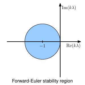
Forward Euler
Use Forward Euler in time \(\Longrightarrow\) FTCS scheme: \[\begin{aligned} U_j^{n+1} = U_j^n - \frac{ak}{2h}\left(U_{j+1}^n - U_{j-1}^n \right) \end{aligned}\]
Stability region \(\mathcal{S}\): \(|1+k\lambda| \le 1\) \(\Longrightarrow\) imaginary \(k\lambda_p\) will always be outside \(\mathcal{S}\) \(\Longrightarrow\) unstable for fixed \(k/h\)
However, if e.g. \(k=h^2\), we have \[\begin{aligned} |1+k\lambda_p|^2 \le 1 + \left( \frac{ka}{h} \right)^2 \\ = 1+a^2h^2 = 1+a^2k \end{aligned}\] which gives Lax-Richtmyer stability \[\begin{aligned} \hspace{-5mm} \|(I+kA)^n\|_2 \le (1+a^2k)^{n/2} \le e^{a^2T/2} \end{aligned}\]
Not used in practice – too strong restriction on timestep \(k\)
Leapfrog
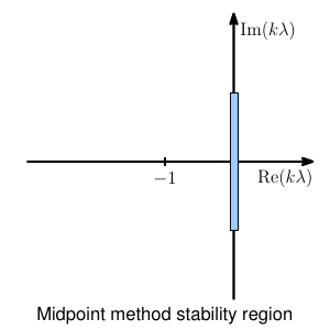
Consider using the midpoint method in time: \[\begin{aligned} U^{n+1} = U^{n-1} + 2kAU^n \end{aligned}\]
For the centered differences in space, this gives the leapfrog method: \[\begin{aligned} U_j^{n+1} = U_j^{n-1} - \frac{ak}{h} \left(U_{j+1}^n - U_{j-1}^n \right) \end{aligned}\]
Stability region \(\mathcal{S}\): \(i\alpha\) for \(-1<\alpha<1\) \(\Longrightarrow\) stable if \(|ak/h|<1\)
Only marginally stable \(\Longrightarrow\) nondissipative
Lax-Friedrichs
Rewrite the average as: \[\begin{aligned} \frac12 \left( U_{j-1}^n + U_{j+1}^n \right) = U_j^n + \frac12 \left( U_{j-1}^n -2U_j^n + U_{j+1}^n \right) \end{aligned}\] to obtain \[\begin{aligned} U_j^{n+1} = U_j^n - \frac{ak}{2h}\left(U_{j+1}^n - U_{j-1}^n \right) +\frac12 \left( U_{j-1}^n - 2U_j^n + U_{j+1}^n \right) \end{aligned}\] or \[\begin{aligned} \frac{U_j^{n+1} - U_j^n}{k} + a \left( \frac{U_{j+1}^n - U_{j-1}^n}{2h} \right) = \frac{h^2}{2k} \left( \frac{U_{j-1}^n - 2U_j^n + U_{j+1}^n}{h^2} \right) \end{aligned}\]
Like a discretization of the advection-diffusion equation \[\begin{aligned} u_t + au_x = \epsilon u_{xx} \end{aligned}\] where \(\epsilon = h^2/(2k)\).
Lax-Friedrichs
The Lax-Friedrichs method can then be written as \(U'(t) = A_\epsilon U(t)\) with \[\begin{aligned} A_\epsilon = -\frac{a}{2h} & \begin{bmatrix} 0 & 1 & & & & -1 \\ -1 & 0 & 1 & & & \\ & -1 & 0 & 1 & & \\ & & \ddots & \ddots & \ddots & \\ & & & -1 & 0 & 1 \\ 1 & & & & -1 & 0 \end{bmatrix} \\ +\frac{\epsilon}{h^2} & \begin{bmatrix} -2 & 1 & & & & 1 \\ 1 & -2 & 1 & & & \\ & 1 & -2 & 1 & & \\ & & \ddots & \ddots & \ddots & \\ & & & 1 & -2 & 1 \\ 1 & & & & 1 & -2 \end{bmatrix} \end{aligned}\] where \(\epsilon=h^2/(2k)\)
Lax-Friedrichs
The eigenvalues of \(A_\epsilon\) are shifted from the imaginary axis into the left half-plane: \[\begin{aligned} \mu_p = -\frac{ia}{h}\sin(2\pi p h) - \frac{2\epsilon}{h^2}(1-\cos(2\pi p h )) \end{aligned}\]
The values \(k\mu_p\) lie on an ellipse centered at \(-2k\epsilon/h^2\), with semi-axes \(2k\epsilon/h^2\), \(ak/h\)
For Lax-Friedrichs, \(\epsilon = h^2/(2k)\) and \(-2k\epsilon/h^2 = -1\) \(\Longrightarrow\) stable if \(|ak/h|\le 1\)
The Lax-Wendroff Method
Use Taylor series method for higher order accuracy in time
For \(U'(t) = AU(t)\), we have \(U''=AU'=A^2U\) and the second-order Taylor method \[\begin{aligned} U^{n+1} = U^n + kAU^n + \frac12 k^2 A^2 U^n \end{aligned}\]
Note that \[\begin{aligned} (A^2U)_j = \frac{a^2}{4h^2} \left( U_{j-2} - 2U_j + U_{j+2} \right) \end{aligned}\] so the method can be written \[\begin{aligned} U_j^{n+1} = U_j^n - \frac{ak}{2h} \left(U_{j+1}^n - U_{j-1}^n \right) + \frac{a^2k^2}{8h^2}\left( U_{j-2}^n - 2U_j^n + U_{j+2}^n \right) \end{aligned}\]
Replace last term by 3-point discretization of \(a^2k^2u_{xx}/2\) \(\Longrightarrow\) the Lax-Wendroff method: \[\begin{aligned} U_j^{n+1} = U_j^n - \frac{ak}{2h} \left(U_{j+1}^n - U_{j-1}^n \right) + \frac{a^2k^2}{2h^2}\left( U_{j-1}^n - 2U_j^n + U_{j+1}^n \right) \end{aligned}\]
Stability analysis
The Lax-Wendroff method is Euler’s method applied to \(U'(t)=A_\epsilon U(t)\), with \(\epsilon=a^2k/2\) \(\Longrightarrow\) eigenvalues \[\begin{aligned} k\mu_p = -i\left( \frac{ak}{h} \right) \sin(p\pi h) + \left( \frac{ak}{h} \right)^2 (\cos(p\pi h) - 1) \end{aligned}\]
On ellipse centered at \(-(ak/h)^2\) with semi-axes \((ak/h)^2\), \(|ak/h|\)
Stable if \(|ak/h|\le 1\)
Upwind methods
Consider one-sided approximations for \(u_x\), e.g. for \(a>0\): \[\begin{aligned} U_j^{n+1} = U_j^n - \frac{ak}{h}(U_j^n - U_{j-1}^n),\text{ stable if } 0\le \frac{ak}{h}\le 1 \end{aligned}\] or, if \(a<0\): \[\begin{aligned} U_j^{n+1} = U_j^n - \frac{ak}{h}(U_{j+1}^n - U_j^n),\text{ stable if } -1\le \frac{ak}{h}\le 0 \end{aligned}\]
Natural with asymmetry for the advection equation, since the solution is translating at speed \(a\)
Stability analysis
The upwind method for \(a>0\) can be written \[\begin{aligned} U_j^{n+1} = U_j^n - \frac{ak}{2h} (U_{j+1}^n - U_{j-1}^n) +\frac{ak}{2h}(U_{j+1}^n - 2U_j^n + U_{j-1}^n) \end{aligned}\]
Again like a discretization of advection-diffusion \(u_t+au_x = \epsilon u_{xx}\), with \(\epsilon=ah/2\) \(\Longrightarrow\) stable if \[\begin{aligned} -2 < -2\epsilon k/h^2<0,\quad\text{or}\quad 0\le \frac{ak}{h} \le 1 \end{aligned}\]
The three methods, Lax-Wendroff, upwind, Lax-Friedrichs, can all be written as advection-diffusion with \[\begin{aligned} \epsilon_{LW} = \frac{a^2k}{2}=\frac{ah\nu}{2},\quad \epsilon_{up} = \frac{ah}{2},\quad \epsilon_{LF} = \frac{h^2}{2k} = \frac{ah}{2\nu} \end{aligned}\] where \(\nu=ak/h\). Stable if \(0<\nu<1\).
The Beam-Warming method
Like upwind, but use second-order one-sided approximations: \[\begin{aligned} U_j^{n+1} = &U_j^n - \frac{ak}{2h}(3U_j^n-4U_{j-1}^n+U_{j-2}^n) \\ & +\frac{a^2k^2}{2h^2}(U_j^n-2U_{j-1}^n+U_{j-2}^n)\quad\text{for } a>0 \end{aligned}\] and \[\begin{aligned} U_j^{n+1} = &U_j^n - \frac{ak}{2h}(-3U_j^n+4U_{j+1}^n-U_{j+2}^n) \\ & +\frac{a^2k^2}{2h^2}(U_j^n-2U_{j+1}^n+U_{j+2}^n)\quad\text{for } a<0 \end{aligned}\]
Stable if \(0\le\nu\le 2\) and \(-2\le\nu\le 0\), respectively
Von Neumann analysis
\[\begin{aligned} g(\xi) = (1-\nu) + \nu e^{-i\xi h} \end{aligned}\] where \(\nu=ak/h\), stable if \(0\le \nu \le 1\)
\[\begin{aligned} g(\xi) = \cos(\xi h) -\nu i \sin(\xi h) &\Longrightarrow |g(\xi)|^2 = \cos^2(\xi h) + \nu^2 \sin^2(\xi h), \end{aligned}\] stable if \(|\nu|\le 1\)
Von Neumann analysis
\[\begin{aligned} g(\xi) = 1-i\nu[2\sin(\xi h/2)\cos(\xi h/2)] - \nu^2[2\sin^2(\xi h/2)] \\ \Longrightarrow |g(\xi)|^2 = 1-4\nu^2(1-\nu^2)\sin^4(\xi h/2) \end{aligned}\] stable if \(|\nu|\le 1\)
\[\begin{aligned} g(\xi)^2 = 1-2\nu i \sin(\xi h) g(\xi), \end{aligned}\] stable if \(|\nu|<1\) (like the midpoint method)
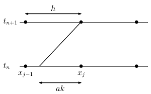
Characteristic tracing and interpolation
Consider the case \(a>0\) and \(ak/h<1\)
Trace characteristic through \(x_j,t_{n+1}\) to time \(t_n\)
Find \(U_j^{n+1}\) by linear interpolation between \(U_{j-1}^n\) and \(U_j^n\): \[\begin{aligned} U_j^{n+1} = U_j^n - \frac{ak}{h} (U_j^n - U_{j-1}^n) \end{aligned}\] \(\Longrightarrow\) first order upwind method
Quadratic interpolating \(U_{j-1}^n\), \(U_j^n\), \(U_{j+1}^n\) \(\Longrightarrow\) Lax-Wendroff
Quadratic interpolating \(U_{j-2}^n\), \(U_{j-1}^n\), \(U_{j}^n\) \(\Longrightarrow\) Beam-Warming
The CFL condition
For the advection equation, \(u(X,T)\) depends only on the initial data \(\eta(X-aT)\)
The domain of dependence is \(\mathcal{D}(X,T) = \{X-aT\}\)
Heat equation \(u_t=u_{xx}\), \(\mathcal{D}(X,T) = (-\infty,\infty)\)
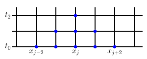
Domain of dependence for 3-point explicit FD method: Each value depends on neighbors at previous timestep
Refining the grid with fixed \(k/h\equiv r\) gives same interval
This region must contain the true \(\mathcal{D}\) for the PDE: \[\begin{aligned} X-T/r\le X-aT \le X+T/r \end{aligned}\] \(\Longrightarrow\) \(|a|\le 1/r\) or \(|ak/h|\le 1\)
The Courant-Friedrichs-Lewy (CFL) condition: Numerical domain of dependence must contain the true \(\mathcal{D}\) as \(k,h\rightarrow 0\)
The CFL condition
The centered-difference scheme for the advection equation is unstable for fixed \(k/h\) even if \(|ak/h|\le 1\)
3-point one-sided stencil, CFL condition gives \(0\le ak/h\le 2\) (for left-sided, used when \(a>0\))
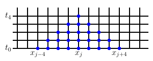
\(\mathcal{D}(X,T) = (-\infty,\infty)\) \(\Longrightarrow\) any 3-point explicit method violates CFL condition for fixed \(k/h\)
However, with \(k/h^2\le 1/2\), all of \(\mathbb{R}\) is covered as \(k\rightarrow 0\)
Any implicit scheme satisfies the CFL condition, since the tridiagonal linear system couples all points.
Modified equations
Find a PDE \(v_t=\cdots\) that the numerical approximation \(U_j^n\) satisfies exactly, or at least better than the original PDE
To second order accuracy, the numerical solution satisfies \[\begin{aligned}
v_t + av_x = \frac12 a h \left( 1 - \frac{ak}{h} \right) v_{xx}
\end{aligned}\]
Advection-diffusion equation
To third order accuracy, \[\begin{aligned}
v_t + av_x + \frac16 ah^2\left( 1- \left(\frac{ak}{h}\right)^2 \right)
v_{xxx} = 0
\end{aligned}\]
Dispersive behavior, leading to a phase error. To
fourth order, \[\begin{aligned}
v_t + av_x + \frac16 ah^2\left( 1- \left(\frac{ak}{h}\right)^2 \right)
v_{xxx} = -\epsilon v_{xxxx}
\end{aligned}\]
where \(\epsilon=O(k^3+h^3)\) \(\Longrightarrow\) highest modes damped
Modified equations
To third order, \[\begin{aligned} v_t + av_x = \frac16 a h^2 \left(2-\frac{3ak}{h}+\left(\frac{ak}{h}\right)^2\right) v_{xxx} \end{aligned}\] Dispersive, similar to Lax-Wendroff
Modified equation \[\begin{aligned} v_t + av_x + \frac16 ah^2\left(1-\left(\frac{ak}{h}\right)^2\right) v_{xxx} = \epsilon v_{xxxxx} + \cdots \end{aligned}\] where \(\epsilon=O(h^4+k^4)\) \(\Longrightarrow\) only odd-order derivatives, nondissipative method
Hyperbolic systems
The methods generalize to first order linear systems of equations of the form \[\begin{aligned} &u_t + Au_x = 0, \\ &u(x,0) = \eta(x), \end{aligned}\]
where \(u : \mathbb{R} \times \mathbb{R} \rightarrow \mathbb{R}^s\) and a constant matrix \(A\in\mathbb{R}^{s\times s}\)Hyperbolic system of conservation laws, with flux function \(f(u)=Au\), if \(A\) diagonalizable with real eigenvalues: \[\begin{aligned} A=R\Lambda R^{-1}\quad\text{or}\quad Ar_p = \lambda_p r_p\text{ for }p=1,2,\ldots,s \end{aligned}\]
Change variables to eigenvectors, \(w=R^{-1}u\), to decouple system into \(s\) independent scalar equations \[\begin{aligned} (w_p)_t + \lambda_p (w_p)_x = 0,\quad p=1,2,\ldots, s \end{aligned}\]
with solution \(w_p(x,t) = w_p(x-\lambda_p t,0)\) and initial condition the \(p\)th component of \(w(x,0)=R^{-1}\eta(x)\).Solution recovered by \(u(x,t) = Rw(x,t)\), or \[\begin{aligned} u(x,t) = \sum_{p=1}^s w_p(x-\lambda_p t, 0)r_p \end{aligned}\]
Numerical methods for hyperbolic systems
Most methods generalize to systems by replacing \(a\) with \(A\)
\[\begin{aligned} U_j^{n+1} = U_j^n - \frac{k}{2h} A(U_{j+1}^n - U_{j-1}^n) + \frac{k^2}{2h^2} A^2 (U_{j-1}^n - 2U_j^n + U_{j+1}^n) \end{aligned}\] Second-order accurate, stable if \(\nu = \max_{1\le p \le s} |\lambda_p k/h| \le 1\)
\[\begin{aligned} U_j^{n+1} &= U_j^n - \frac{k}{h} A(U_j^n - U_{j-1}^n) \\ U_j^{n+1} &= U_j^n - \frac{k}{h} A(U_{j+1}^n - U_{j}^n) \end{aligned}\] Only useful if all eigenvalues of \(A\) have same sign. Instead, decompose into scalar equations and upwind each one separately \(\Longrightarrow\) Godunov’s method
Initial boundary value problems
For a bounded domain, e.g. \(0\le x \le 1\), the advection equation requires an inflow condition \(x(0,t)=g_0(t)\) if \(a>0\)
This gives the solution \[\begin{aligned} u(x,t) = \begin{cases} \eta(x-at) & \text{if }0\le x-at\le 1, \\ g_0(t-x/a) & \text{otherwise}. \end{cases} \end{aligned}\]
First-order upwind works well, but other stencils need special cases at inflow boundary and/or outflow boundary
von Neumann analysis not applicable, but generally gives necessary conditions for convergence
Method of Lines applicable if eigenvalues of discretization matrix are known