The Level Set Method
Math 228B Numerical Solutions of Differential Equations
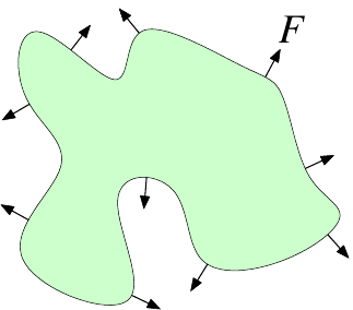
Evolving Curves and Surfaces
Propagate curve according to speed function \(\boldsymbol{v}=F\boldsymbol{n}\)
\(F\) depends on space, time, and the curve itself
Surfaces in three dimensions
Geometry Representations
Explicit Geometry
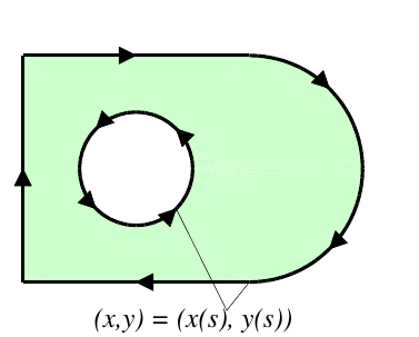
Parameterized boundaries
Implicit Geometry
Boundaries given by zero levelset
Explicit Techniques
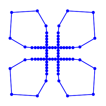
Simple approach: Represent curve explicitly by a set of nodes \(\{\boldsymbol{x}^{(i)}\}\), connected by lines or splines
Propagate curve by solving ODEs \[\begin{aligned} \frac{d\boldsymbol{x}^{(i)}}{dt} = \boldsymbol{v}(\boldsymbol{x}^{(i)},t),\quad \boldsymbol{x}^{(i)}(0) = \boldsymbol{x}^{(i)}_0, \end{aligned}\]
Calculate normal vectors, curvatures, etc by difference approximations, e.g.: \[\begin{aligned} \frac{d\boldsymbol{x}^{(i)}}{ds}\approx \frac{\boldsymbol{x}^{(i+1)}-\boldsymbol{x}^{(i-1)}}{2\Delta s} \end{aligned}\]
MATLAB Demo
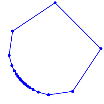
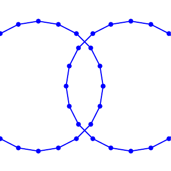
Explicit Techniques - Drawbacks
Node redistribution required, introduces errors
No entropy solution, sharp corners handled incorrectly
Need special treatment for topology changes
Stability constraints for curvature dependent speed functions
Node distribution
Sharp corners
Topology changes
The Level Set Method
Implicit geometries, evolve interface by solving PDEs
Invented in 1988 by Osher and Sethian:
Stanley Osher and James A. Sethian. Fronts propagating with curvature-dependent speed: algorithms based on Hamilton- Jacobi formulations. J. Comput. Phys., 79(1):12–49, 1988.
Introductory books:
James A. Sethian. Level set methods and fast marching methods. Cambridge University Press, Cambridge, second edition, 1999.
Stanley Osher and Ronald Fedkiw. Level set methods and dynamic implicit surfaces. Springer-Verlag, New York, 2003.
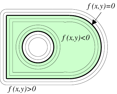
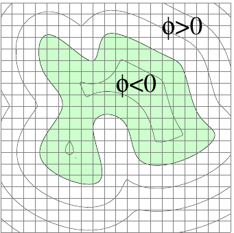
Implicit Geometries
Represent curve by zero level set of a function, \(\phi(\boldsymbol{x})=0\)
Special case: Signed distance function:
\(|\nabla\phi|=1\)
\(|\phi(\boldsymbol{x})|\) gives (shortest) distance from \(\boldsymbol{x}\) to curve
Discretized Implicit Geometries
Discretize implicit function \(\phi\) on background grid
Obtain \(\phi(\boldsymbol{x})\) for general \(\boldsymbol{x}\) by interpolation
Cartesian 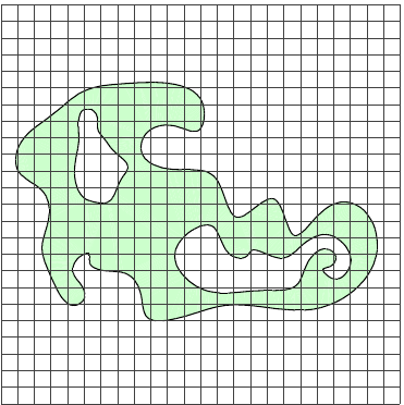
Quadtree/Octree 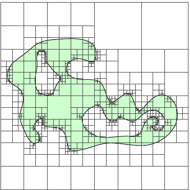
Geometric Variables
Normal vector \(\boldsymbol{n}\) (without assuming distance function): \[\begin{aligned} \boldsymbol{n}=\frac{\nabla\phi}{|\nabla\phi|} \end{aligned}\]
Curvature (in two dimensions): \[\begin{aligned} \kappa=\nabla\cdot \frac{\nabla \phi}{|\nabla \phi|} = \frac{\phi_{xx}\phi_y^2-2\phi_y\phi_x\phi_{xy}+\phi_{yy}\phi_x^2}{(\phi_x^2+\phi_y^2)^{3/2}}. \end{aligned}\]
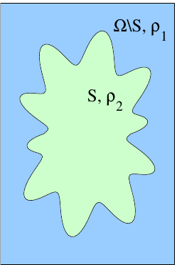
Write material parameters, etc, in terms of \(\phi\): \[\begin{aligned} \rho(\boldsymbol{x}) = \rho_1 + (\rho_2-\rho_1)\theta(\phi(\boldsymbol{x})) \end{aligned}\] Smooth Heaviside function \(\theta\) over a few grid cells.
The Level Set Equation
Solve convection equation to propagate \(\phi=0\) by velocities \(\boldsymbol{v}\) \[\begin{aligned} \phi_t + \boldsymbol{v}\cdot \nabla\phi = 0. \end{aligned}\]
For \(\boldsymbol{v}=F\boldsymbol{n}\), use \(\boldsymbol{n}=\nabla\phi/|\nabla\phi|\) and \(\nabla\phi\cdot\nabla\phi=|\nabla\phi|^2\) to obtain the Level Set Equation \[\begin{aligned} \phi_t+F|\nabla\phi|=0. \end{aligned}\]
Nonlinear, hyperbolic equation (Hamilton-Jacobi).
Discretization
Use upwinded finite difference approximations for convection
For the level set equation \(\phi_t+F|\nabla\phi|=0\): \[\begin{aligned} \phi_{ijk}^{n+1}\ &= \phi_{ijk}^n - \Delta t \left( \max(F,0)\nabla^{+}_{ijk} + \min(F,0)\nabla^{-}_{ijk} \right), \end{aligned}\] where \[\begin{aligned} \nabla^{+}_{ijk} = \big[ & \max(D^{-x}\phi_{ijk}^n,0)^2+ \min(D^{+x}\phi_{ijk}^n,0)^2 + \nonumber \\ & \max(D^{-y}\phi_{ijk}^n,0)^2+ \min(D^{+y}\phi_{ijk}^n,0)^2 + \nonumber \\ & \max(D^{-z}\phi_{ijk}^n,0)^2+ \min(D^{+z}\phi_{ijk}^n,0)^2 \big] ^{1/2}, \end{aligned}\]
Discretization
and \[\begin{aligned} \nabla^{-}_{ijk} = \big[ & \min(D^{-x}\phi_{ijk}^n,0)^2+ \max(D^{+x}\phi_{ijk}^n,0)^2 + \nonumber \\ & \min(D^{-y}\phi_{ijk}^n,0)^2+ \max(D^{+y}\phi_{ijk}^n,0)^2 + \nonumber \\ & \min(D^{-z}\phi_{ijk}^n,0)^2+ \max(D^{+z}\phi_{ijk}^n,0)^2 \big] ^{1/2}. \end{aligned}\]
\(D^{-x}\) backward difference operator in the \(x\)-direction, etc
For curvature dependent part of \(F\), use central differences
Higher order schemes available
MATLAB Demo
Reinitialization
Even if the initial level set function is a distance function, general speed functions \(F\) will give large variations in \(|\nabla\phi|\)
This gives poor accuracy and performance, and requires smaller timesteps for stability
Reinitialize the level set function by finding a new \(\phi\) with same zero level set but \(|\nabla\phi|=1\)
Different approaches:
Integrate the reinitialization equation for a few time steps \[\begin{aligned} \phi_t + \mathrm{sign}(\phi) ( |\nabla \phi| - 1 ) = 0 \end{aligned}\]
Compute distances from \(\phi=0\) explicitly for nodes close to boundary, use Fast Marching Method for remaining nodes
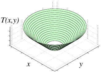
The Boundary Value Formulation
For \(F>0\), formulate evolution by an arrival function \(T\)
\(T(\boldsymbol{x})\) gives time to reach \(\boldsymbol{x}\) from initial \(\Gamma\)
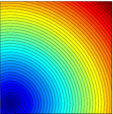
time * rate = distance gives the Eikonal equation: \[\begin{aligned} |\nabla T|F = 1, \quad T=0\text{ on }\Gamma. \end{aligned}\]
Special case: \(F=1\) gives distance functions
The Fast Marching Method
Discretize the Eikonal equation \(|\nabla T|F=1\) by \[\begin{aligned} \left[ \begin{array}{r} \max(D_{ijk}^{-x}T,0)^2+\min(D_{ijk}^{+x}T,0)^2 \\ +\max(D_{ijk}^{-y}T,0)^2+\min(D_{ijk}^{+y}T,0)^2 \\ +\max(D_{ijk}^{-z}T,0)^2+\min(D_{ijk}^{+z}T,0)^2 \\ \end{array} \right]^{1/2} = \frac{1}{F_{ijk}} \end{aligned}\] or \[\begin{aligned} \label{fmmdisc} \left[ \begin{array}{r} \max(D_{ijk}^{-x}T,-D_{ijk}^{+x}T,0)^2 \\ +\max(D_{ijk}^{-y}T,-D_{ijk}^{+y}T,0)^2 \\ +\max(D_{ijk}^{-z}T,-D_{ijk}^{+z}T,0)^2 \\ \end{array} \right]^{1/2} = \frac{1}{F_{ijk}} \end{aligned}\]
The Fast Marching Method
Use the fact that the front propagates outward
Tag known values and update neighboring \(T\) values (using the difference approximation)
Pick unknown with smallest \(T\) (will not be affected by other unknowns)
Update new neighbors and repeat until all nodes are known
Store unknowns in priority queue, \(\mathcal{O}(n\log n)\) performance for \(n\) nodes with heap implementation
Application: First arrivals and shortest geodesic paths
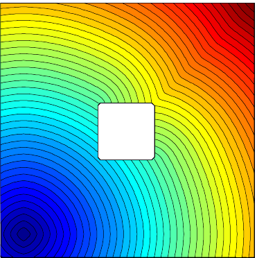
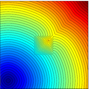
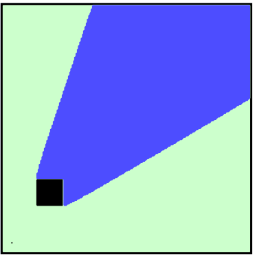
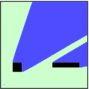
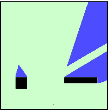
Visibility around obstacles
Application: Structural Vibration Control
Consider eigenvalue problem \[\begin{aligned} -\Delta u &= \lambda \rho(\boldsymbol{x})u, & x &\in \Omega \\ u &= 0, & x &\in \partial \Omega. \text{with} \rho(\boldsymbol{x}) &= \begin{cases} \rho_1 & \textrm{for }x \notin S \\ \rho_2 & \textrm{for }x \in S. \end{cases} \end{aligned}\]
Solve the optimization \[\begin{aligned} \min_S \lambda_1 \textrm{ or } \lambda_2 \textrm{ subject to } \|S\|=K. \end{aligned}\]
Application: Structural Vibration Control
Level set formulation by Osher and Santosa:
Finite difference approximations for Laplacian
Sparse eigenvalue solver for solutions \(\lambda_i, u_i\)
Calculate descent direction \(\delta \phi=-v(\boldsymbol{x})|\nabla \phi|\) with \(v(\boldsymbol{x})\) from shape sensitivity analysis
Find a Lagrange multiplier that enforces the area constraint using Newton’s method
Represent interface implicitly, propagate using level set method