Mesh Generation
Math 228B Numerical Solutions of Differential Equations
Mesh Generation
Motivation: Most numerical methods for
PDEs require a mesh for non-trivial domains
Various methods might use different components of the mesh:
Nodes (vertices)
Edges (faces in 3D)
Elements
Structured vs. Unstructured Meshes
Natural classification of meshes based on connectivity of nodes:
In structured meshes, all nodes have the same connections to their neighbors (at least away from the boundaries)
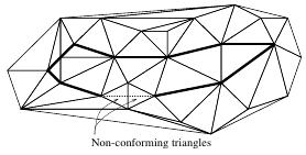
Unstructured meshes allow for arbitrary connectivities (as long as the mesh remains conforming)
Hybrid meshes combine the two, e.g. by having structured parts in certain areas of the domain
Structured Mesh Generation
Why Structured Meshes?
Lead to very efficient numerical methods
High quality for sufficiently simple geometries
Larger grid control when high anisotropy is required
Multi-block approach allows for realistic geometries
Single-Block Grid Generation
Construct a one-to-one mapping between a rectangular computational domain and a physical domain
Ideally, grid size in physical space should be dictated by solver/solution requirements
Ensure grid quality e.g. smoothness, orthogonality
Single Block Grid Generation - Creating the Mapping
Transfinite Interpolation (TFI)
Conformal Mapping
Solving PDE’s
Elliptic
Parabolic/Hyperbolic
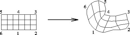
Algebraic Mappings
Construct a mapping between the boundaries of the unit square (cube) and the boundaries of an "arbitrary" region which is topologically equivalent
Combine 1D interpolants using Boolean sums to construct mapping - Transfinite Interpolation (TFI)
Not guaranteed to be one-to-one
Orthogonality not guaranteed
Very Fast
Quite General
Grid quality not always assured
Algebraic Mappings - 1D Interpolants
General 1D interpolant of \(f(x)\) for \(x \in (0,1)\) \[\hat{f}(x) \equiv \Pi_x f = \sum_{i=0}^L \sum_{n=0}^P \alpha^n_i(x) \left. \frac{d^n f}{d x^n} \right|_{x=x_i}\]
\(\alpha^n_i(x)\) are the blending functions
Examples
Linear Lagrange interpolation - \(P=0, L=1\) \[\Pi_x f = (1-x) f(0) + x f(1)\]
Quadratic Lagrange interpolation - \(P=0, L=2\) \[\Pi_x f = (2x^2 - 3x + 1) f(0)+ (4x-4x^2)f(0.5) + (2x^2-x) f(1)\]
Hermite interpolation - \(P=1, L=1\) \[\begin{aligned} \Pi_x f & = & (2x^3-3x^2+1)f(0) + (3x^2-2x^3) f(1) + \\ & & (x^3-2x^2+x) f'(0) + (x^3-x^2) f'(1) \end{aligned}\]
Algebraic Mappings - Transfinite Interpolation
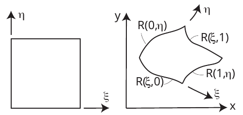
Start from 1D boundary mappings of \({\bf R}\equiv (x,y)\), e.g.
\({\bf R}(\xi,0), {\bf R}(\xi,1), {\bf R}(0,\eta), {\bf R}(1,\eta)\)
Construct 1D interpolants in the \(\xi\) and \(\eta\) directions (e.g. linear) \[\begin{aligned} \Pi_\xi {\bf R} & = & (1-\xi){\bf R}(0,\eta) + \xi {\bf R}(1,\eta) \\ \Pi_\eta {\bf R} & = & (1-\eta){\bf R}(\xi,0) + \eta {\bf R}(\xi,1) \end{aligned}\]
Algebraic Mappings - Transfinite Interpolation
Construct two-dimensional interpolant by doing the Boolean sum \[\hat{{\bf R}}(\xi,\eta) = (\Pi_\xi \oplus \Pi_\eta) {\bf R} = (\Pi_{\xi} + \Pi_\eta - \Pi_\xi \Pi_\eta) {\bf R}\] Expanding: \[\hat{{\bf R}}(\xi,\eta) = (1-\xi,\xi)\left(\begin{array}{c} {\bf R}(0,\eta) \\ {\bf R}(1,\eta) \end{array}\right) + ({\bf R}(\xi,0),{\bf R}(\xi,1))\left(\begin{array}{c} 1-\eta \\ \eta \end{array}\right)\] \[- (1-\xi,\xi)\left(\begin{array}{cc} {\bf R}(0,0) & {\bf R}(0,1)\\ {\bf R}(1,0) & {\bf R}(1,1) \end{array}\right)\left(\begin{array}{c} 1-\eta \\ \eta \end{array}\right)\] \[=(1-\xi){\bf R}(0,\eta) + \xi{\bf R}(1,\eta) + (1-\eta){\bf R}(\xi,0) + \eta{\bf R}(\xi,1)\] \[-(1-\xi)(1-\eta){\bf R}(0,0) - (1-\xi)\eta{\bf R}(0,1) - \xi(1-\eta){\bf R}(1,0) -\xi\eta{\bf R}(1,1)\]
Important property: Preserves \({\bf R}\) at the domain boundary
Extends to general 1D interpolants and any dimension
Algebraic Mappings - Example
Algebraic Mappings - Example
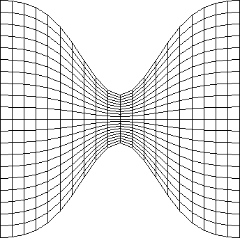
\(\Pi_\xi {\bf R}\)
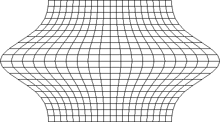
\(\Pi_\eta {\bf R}\)
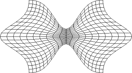
\((\Pi_\xi \oplus \Pi_\eta) {\bf
R}\)
Algebraic Mappings - Grid Control
Use non-regular subdivisions in \((\xi, \eta)\) (e.g. exponential functions) to obtain desired element sizes in \((x,y)\)
Use derivative boundary conditions to enforce boundary orthogonality \[\frac{\partial{\bf R}}{\partial \xi} \cdot \frac{\partial{\bf R}}{\partial \eta} = 0\]
Conformal Mapping
An analytic function \(\alpha = f (z)\) such that \(\displaystyle \frac{df}{dz} \ne 0\) defines a one-to-one (conformal) mapping between \(z = x + i y\) and \(\alpha = \xi + i \eta\), or between \((x,y)\) and \((\xi, \eta)\).
The functions \(\xi(x,y)\) and \(\eta(x,y)\) satisfy the Cauchy- Riemann equations (e.g. \(\xi_x=\eta_y\), and \(\eta_x= - \xi_y\)) and as a consequence, they are harmonic \[\nabla^2 \xi = 0, \qquad \nabla^2 \eta = 0 \qquad \mbox{(smoothness)}\]
Preserve angles (grid orthogonality)
Preserve ratios
Lead to high quality grids
Limited to 2D
Conformal Mapping Transformations
Joukowski (maps circle of radius \(c\) to segment \([-2c, 2c]\)) \[\alpha = z + \frac{c^2}{z}, \quad \mbox{or} \qquad \frac{\alpha + 2c}{\alpha-2c} = \left(\frac{z+c}{z-c}\right)^2\]
Karman-Trefftz \[\frac{\alpha + 2c}{\alpha-2c} = \left(\frac{z+c}{z-c}\right)^n\]
Schwarz-Christoffel (maps polygon into half plane) \[\frac{d \alpha}{dz} = K\prod_{k=1}^n\left( 1-\frac{z}{z_k}\right)^{\beta_k}\]
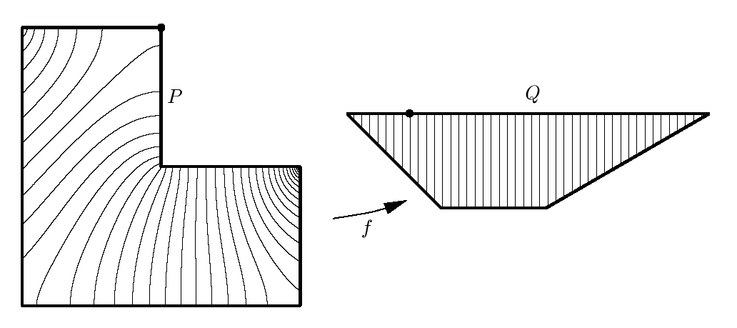
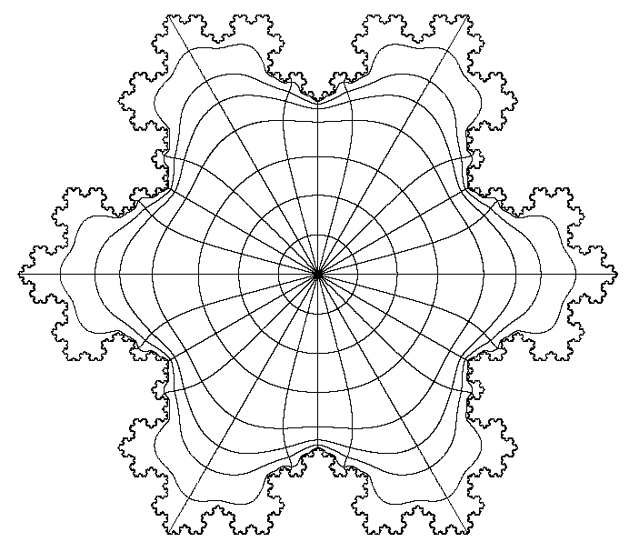
Conformal Mapping - Schwarz-Christoffel
Ref. “Schwarz-Christofell Mapping”, Driscoll and Trefethen, Cambridge Univeristy Press, 2002.
 |
 |
PDE Grid Generation
Construct mapping by solving a PDE
Elliptic Equations (smooth grids) \[\nabla^2 \xi (x,y) = P(x,y), \quad \nabla^2\eta(x,y) = Q(x,y)\]
Hyperbolic equations (orthogonal grids) \[\begin{aligned} x_\xi y_\eta - x_\eta y_\xi & =& J \qquad \mbox{(size control)}\\ x_\xi x_\eta + y_\xi y_\eta & = & 0 \qquad \mbox{(orthogonality)} \end{aligned}\]
Most widely used approach
Grids usually have high quality
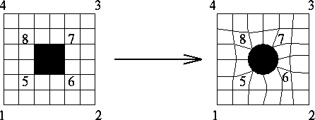
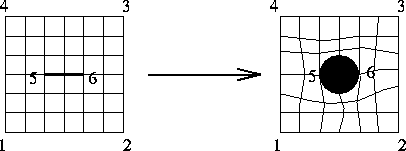
Elliptic Grid Generation
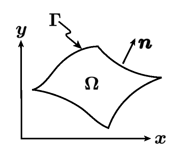
We are interested in solving \[\begin{array}{rcll} - \nabla^2 \xi & = & P & \qquad \mbox{in} \quad \Omega \\[2ex] \xi & = & g & \qquad \mbox{on} \quad \Gamma_D \\[2ex] \displaystyle \frac{\partial \xi}{\partial n} & = & h & \qquad \mbox{on} \quad \Gamma_N = \Gamma \backslash \Gamma_D \end{array}\]
where \(P\), \(g\), and \(h\) are given.
Similarly for \(\eta(x,y)\)
Elliptic Grid Generation
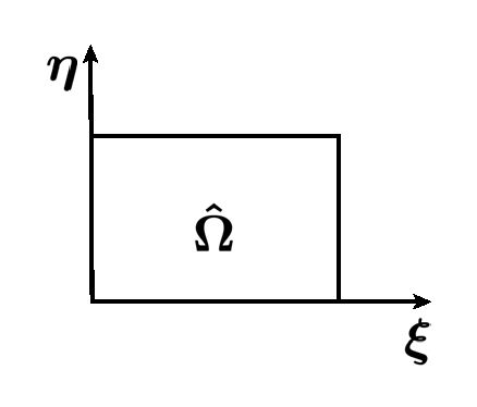
? ?
\[\begin{array}{c} x = x (\xi, \eta)\\ y = y (\xi, \eta)\\ \longrightarrow \end{array}\]
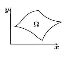
\(\nabla^2 \xi = P\)
Can we determine an equivalent problem to be solved on \(\hat{\Omega}\)?
Elliptic Grid Generation
\(\displaystyle \begin{array}{ccc} \xi = \xi (x,y) & & x = x (\xi, \eta)\\ \eta = \eta (x,y) & & y = y (\xi, \eta)\\ & & \ \ \\ \left( \begin{array}{c} d \xi \\[1.5ex] d \eta \end{array} \right) = \left( \begin{array}{ccc} \xi_x & \ & \xi_y \\[1.5ex] \eta_x & & \eta_y \end{array} \right) \left( \begin{array}{c} d x \\[1.5ex] d y \end{array} \right) & & \left( \begin{array}{c} d x \\[1.5ex] d y \end{array} \right) = \left( \begin{array}{ccc} x_{\xi} & \ & x_{\eta} \\[1.5ex] y_{\xi} & & y_{\eta} \end{array} \right) \left( \begin{array}{c} d \xi \\[1.5ex] d \eta \end{array} \right) \end{array}\)
\(\Rightarrow \displaystyle \left( \begin{array}{ccc} \xi_x & \ & \xi_y \\[1.5ex] \eta_x & & \eta_y \end{array} \right) = \left( \begin{array}{ccc} x_{\xi} & \ & x_{\eta} \\[1.5ex] y_{\xi} & & y_{\eta} \end{array} \right)^{-1} = \frac{1}{J} \left( \begin{array}{ccc} y_{\eta} & \ & - x_{\eta} \\[1.5ex] - y_{\xi} & & x_{\xi} \end{array} \right)\)
\(J = x_{\xi} y_{\eta} - x_{\eta} y_{\xi}\)
Elliptic Grid Generation
\(\begin{array}{rclcrcl} \xi_x & = & \frac{y_\eta}{J} & \quad & \xi_y & = & -\frac{x_\eta}{J}\\[1ex] \eta_x & = & -\frac{y_\xi}{J} & \quad & \eta_y & = & \frac{x_\xi}{J} \end{array}\)
and \(\begin{array}[t]{rcl} \xi_{xx} & = & \displaystyle \frac{\partial}{\partial x} \: (\xi_x) \ = \ \left(\xi_x \: \frac{\partial}{\partial \xi} + \eta_x \: \frac{\partial}{\partial \eta} \right) \left(\frac{y_\eta}{J}\right) \\[1ex] & = & \displaystyle \frac{1}{J} \left( y_{\eta} \: \frac{\partial}{\partial \xi} - y_{\xi} \frac{\partial}{\partial \eta} \right) \left(\frac{y_\eta}{J}\right) \\[1ex] & = & \ldots\\[2ex] \xi_{yy} & = & \ldots \end{array}\)
Elliptic Grid Generation - Thompson’s Equations Finally, \(\xi_{xx} + \xi_{yy} = 0\) and \(\eta_{xx} + \eta_{yy} = 0\), become
\(\fbox{$ \displaystyle \begin{array}{rcl} a x_{\xi\xi} - 2 b x_{\xi \eta} + cx_{\eta\eta} & = & 0 \\ a y_{\xi\xi} - 2 b y_{\xi\eta} + cy_{\eta\eta} & = & 0 \end{array} $}\)
\(a\), \(b\), \(c\) depend on the mapping.
\(\begin{array}{ccc} a = x^2_{\eta} + y^2_{\eta} & b = x_{\xi} x_{\eta} + y_{\xi} y_{\eta} & c = x^2_{\xi} + y^2_{\xi} \end{array}\)
These equations can be solved using central finite differences on a regular grid in the \((\xi, \eta)\) domain to determine the \((x,y)\) coordinates of each grid point.
Picard iteration: Start from initial grid coordinates \(x,y\). Compute \(a,b,c\), solve the PDE, and repeat until convergence.
Elliptic Grid Generation - Grid Control
Modify grid by e.g. adding source terms to the PDE:
\(\xi_{xx} + \xi_{yy} = P(x,y)\) and \(\eta_{xx} + \eta_{yy} = Q(x,y)\)
\(\fbox{$ \displaystyle \begin{array}{rcl} a x_{\xi\xi} - 2 b x_{\xi \eta} + cx_{\eta\eta} & = & -J^2 (x_\xi P + x_\eta Q) \\ a y_{\xi\xi} - 2 b y_{\xi\eta} + cy_{\eta\eta} & = & -J^2 (y_\xi P + y_\eta Q) \end{array} $}\)
The functions \(P(\xi,\eta)\) and \(Q(\xi,\eta)\) can be used to obtain grid control
Derivative boundary conditons can be used to enforce grid orthogonality at the boundary
Ref: “Numerical Generation of Two-Dimensional Grids by Use of Poisson Equations with Grid Control”, Sorenson and Steger, in Numerical Grid Generation Techniques, Smith, R.E. (Ed.), NASA-CP-2166, pp. 449-461, 1980
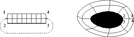
Single-Block Grid Common Topologies
 |
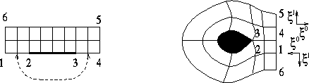 |
| O-Grid | C-Grid |
 |
 |
…plus combinations
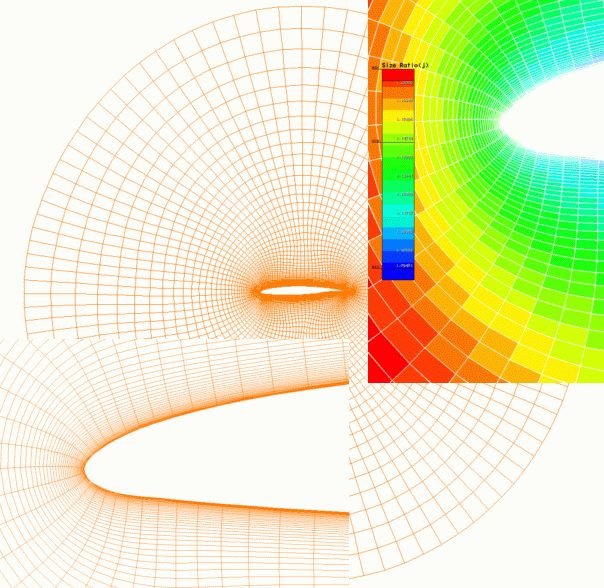
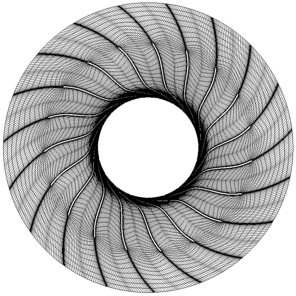
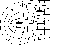
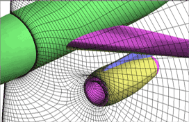
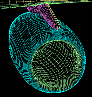
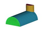
Examples: Single-Block O-Grids
 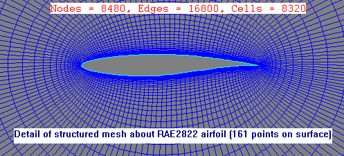 |
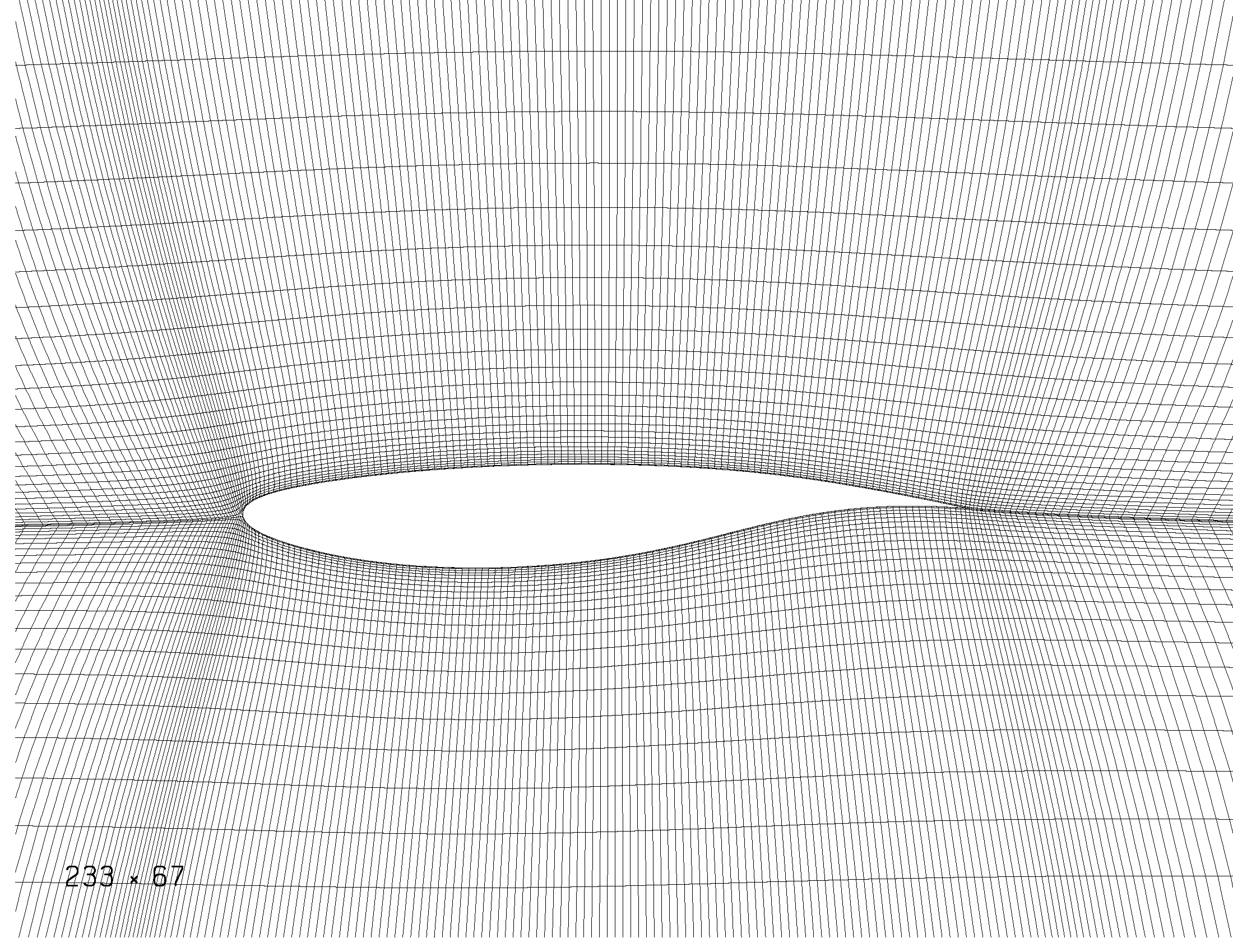
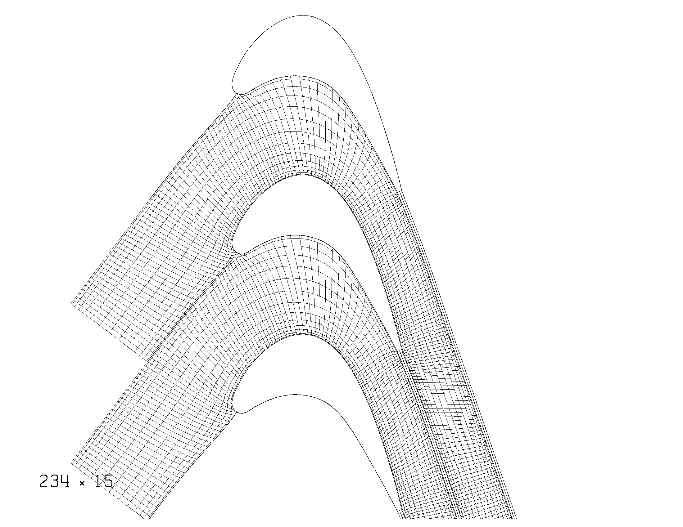
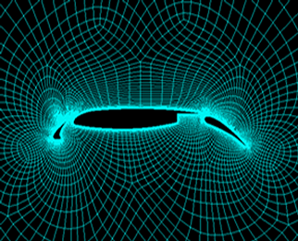
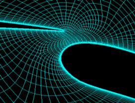
Examples: Single-Block C,H-Grids
  |
 |
 |
 |
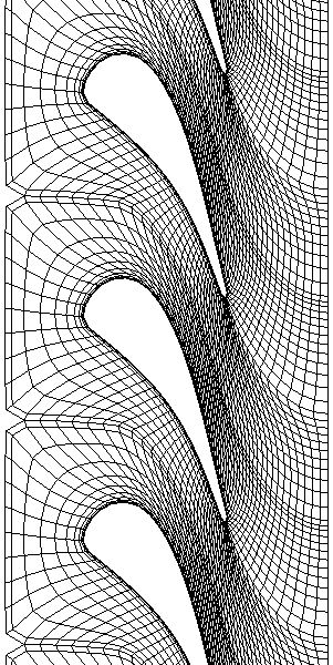
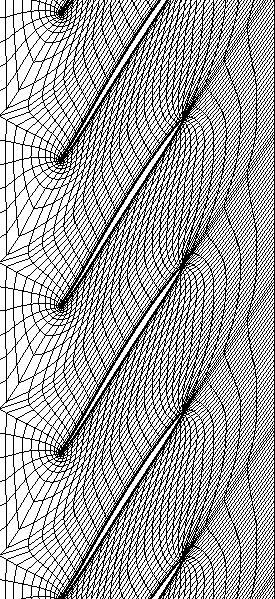
Examples: H-Grids
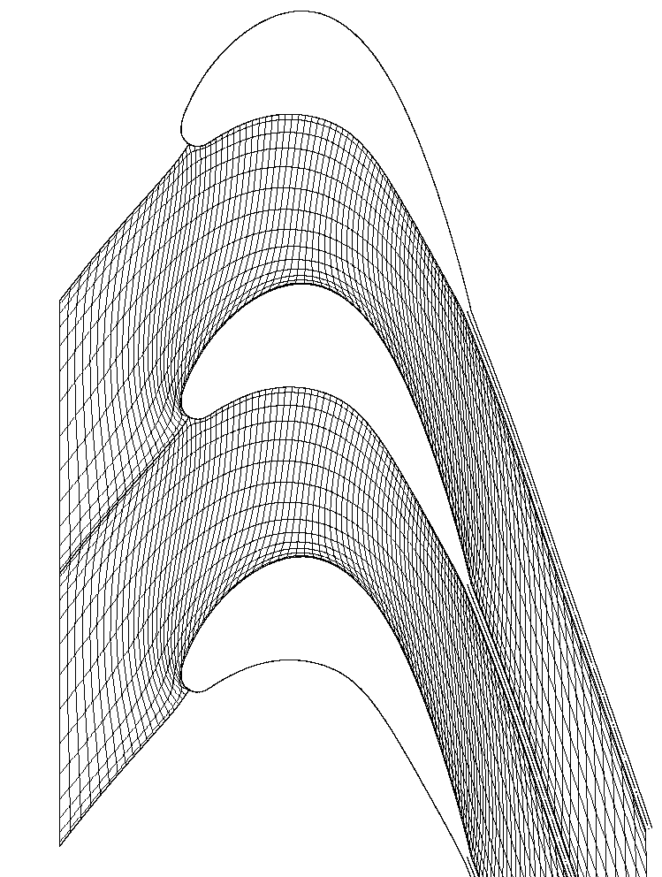 |
 |
| H-Grid | H-Grid/I-Grid |
Multi-Block Grid Generation
Subdivide domain into an unstructured assembly of quadrilaterals/hexahedra
Obtaining block topology automatically is hard
Obtaining block geometry automatically (e.g. point coordinates) once topology is known is tractable
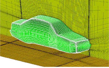
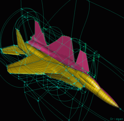
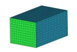
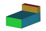
Examples: Multi-Block Grids
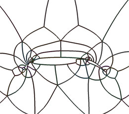 |
 |
|
 |
 |
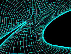
Examples: Multi-Block Grids
 |
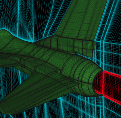 |
 |
 |
Block Topology Generators
(from ICEM CFD)
 |
 |
 |
 |
Automatic \(H \Rightarrow O\) conversion
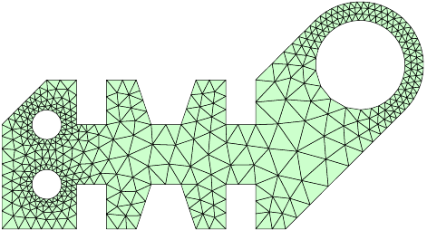
Unstructured Mesh Generation
Unstructured Mesh Generation
Approximate a domain in \(\mathbb{R}^d\) by simple geometric shapes
Determine node points and element connectivity
Goal: Resolve the domain accurately with well-shaped elements, but use as few elements as possible
Applications: Numerical solution of PDEs (FEM, FVM, DGM, BEM), interpolation, computer graphics, visualization
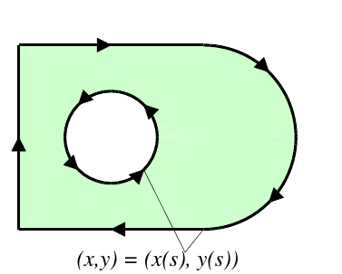
Geometry Representations
Explicit Geometry
Parameterized boundaries
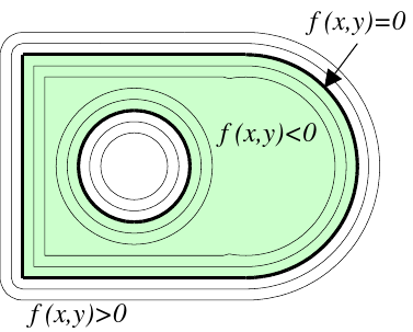
Implicit Geometry
Boundaries from contour
Unstructured Meshing Algorithms
Delaunay refinement
Refine an initial triangulation by inserting centroid points and updating connectivities
Efficient and robust, provably good in 2-D
Advancing front
Propagate a layer of elements from boundaries into domain, stitch together at intersection
High quality meshes, good for boundary layers, but somewhat unreliable in 3-D
Unstructured Meshing Algorithms
Octree mesh
Create an octree, refine until geometry well resolved, form elements between cell intersections
Guaranteed quality even in 3-D, but poor element qualities
DistMesh
Improve initial triangulation by node movements and connectivity updates
Easy to understand and use, handles implicit geometries, high element qualities, but non-robust and low performance
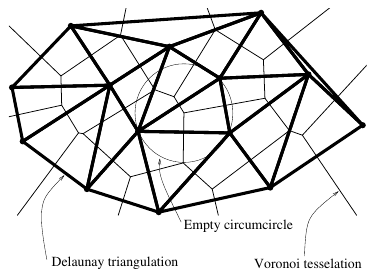
Delaunay Triangulation
Find non-overlapping triangles that fill the convex hull of a set of points
Properties:
Every edge is shared by at most two triangles
The circumcircle of a triangle contains no other input points
Maximizes the minimum angle of all the triangles
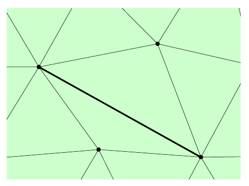
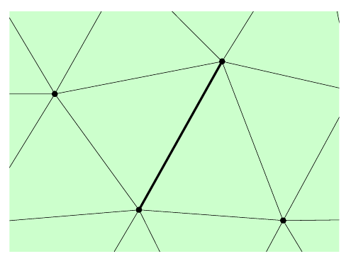
Constrained Delaunay Triangulation
The Delaunay triangulation might not respect given input edges
Use local edge swaps to recover the input edges
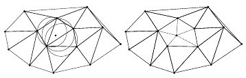
Delaunay Refinement Method
Algorithm:
Form initial triangulation using boundary points and outer box
Replace an undesired element (bad or large) by inserting its circumcenter, retriangulate and repeat until mesh is good
Will converge with high element qualities in 2-D
Very fast – time almost linear in number of nodes
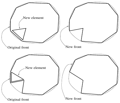
The Advancing Front Method
Discretise the boundary as initial front
Add elements into the domain and update the front
When front is empty the mesh is complete
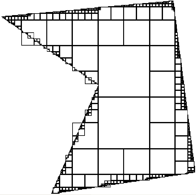
Grid Based and Octree Meshing
Overlay domain with regular grid, crop and warp edge points to boundary
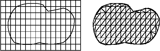
Octree instead of regular grid gives graded mesh with fewer elements
Mesh Size Functions
Function \(h(\boldsymbol{x})\) specifying desired mesh element size
Many mesh generators need a priori mesh size functions
Physically-based methods such as DistMesh
Advancing front and Paving methods
Discretize mesh size function \(h(\boldsymbol{x})\) on a background grid
Mesh Size Functions
Based on several factors:
Curvature of geometry boundary
Local feature size of geometry
Numerical error estimates (adaptive solvers)
Any user-specified size constraints
Also: \(|\nabla h(\boldsymbol{x})|\le g\) to limit ratio \(G=g+1\) of neighboring element sizes
Explicit Mesh Size Functions
A point-source \[\begin{aligned} h(\boldsymbol{x}) = h_\mathrm{pnt} + g |\boldsymbol{x}-\boldsymbol{x}_0| \end{aligned}\]
Any shape, with distance function \(\phi(\boldsymbol{x})\) \[\begin{aligned} h(\boldsymbol{x}) = h_\mathrm{shape} + g \phi(\boldsymbol{x}) \end{aligned}\]
Combine mesh size functions by \(\min\) operator: \[\begin{aligned} h(\boldsymbol{x}) = \min_i h_i(\boldsymbol{x}) \end{aligned}\]
For more general \(h(\boldsymbol{x})\), solve the gradient limiting equation [Persson’05] \[\begin{aligned} \frac{\partial h}{\partial t} + |\nabla h| &= \min (|\nabla h|,g), \\ h(t=0, \boldsymbol{x}) &= h_0(\boldsymbol{x}). \end{aligned}\]
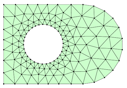
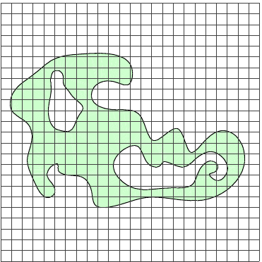
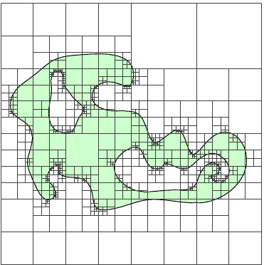
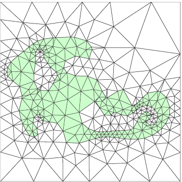
Mesh Size Functions – 2-D Examples
Mesh Size Function \(h(\boldsymbol{x})\)
Mesh Based on \(h(\boldsymbol{x})\)
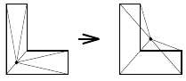
Laplacian Smoothing
Improve node locations by iteratively moving nodes to average of neighbors: \[\begin{aligned} \boldsymbol{x}_i \leftarrow \frac{1}{n_i}\sum_{j=1}^{n_i} \boldsymbol{x}_j \end{aligned}\]
Usually a good postprocessing step for Delaunay refinement
However, element quality can get worse and elements might even invert:
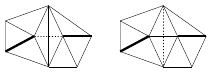
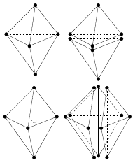
Face and Edge Swapping
In 3-D there are several swappings between neighboring elements
Face and edge swapping important postprocessing of Delaunay meshes
Boundary Layer Meshes
Unstructured mesh for offset curve \(\psi(\boldsymbol{x})-\delta\)
The structured grid is easily created with the distance function

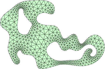
The DistMesh Mesh Generator
The DistMesh Mesh Generator
Start with any topologically correct initial mesh, for example random node distribution and Delaunay triangulation
Move nodes to find force equilibrium in edges
Project boundary nodes using implicit function \(\phi\)
Update element connectivities

Internal Forces

For each interior node: \[\begin{aligned} \sum_i \boldsymbol{F}_i = 0 \end{aligned}\] Repulsive forces depending on edge length \(\ell\) and equilibrium length \(\ell_0\): \[\begin{aligned} |\boldsymbol{F}| = \begin{cases} k(\ell_0-\ell) & \text{if }\ell<\ell_0, \\ 0 & \text{if }\ell\ge\ell_0. \end{cases} \end{aligned}\] Get expanding mesh by choosing \(\ell_0\) larger than desired length \(h\)
Reactions at Boundaries

For each boundary node: \[\begin{aligned} \sum_i \boldsymbol{F}_i + \boldsymbol{R} = 0 \end{aligned}\] Reaction force \(\boldsymbol{R}\):
Orthogonal to boundary
Keeps node along boundary
Node Movement and Connectivity Updates
Move nodes \(\boldsymbol{p}\) to find force equilibrium: \[\begin{aligned} \boldsymbol{p}_{n+1}=\boldsymbol{p}_n+\Delta t \boldsymbol{F}(\boldsymbol{p}_n) \end{aligned}\]
Project boundary nodes to \(\phi(\boldsymbol{p})=0\)
Elements deform, change connectivity based on element quality or in-circle condition (Delaunay)