UC Berkeley Math 228B, Spring 2024, Problem Set 1
Per-Olof Persson
persson@berkeley.edu
Due February 2
This content is protected and may not be shared, uploaded, or distributed.
Show that the 9-point Laplacian in LeVeque (3.17) has the truncation error derived in Section 3.5. Hint: To simplify the computation, note that the 9-point Laplacian can be written as the 5-point Laplacian (with known truncation error) plus a finite difference approximation that models \(\frac 1 6 h^2 u_{xxyy} + O(h^4)\).
Modify the Julia function
assemblePoissonin the Julia notebook on the course webpage, to use the 9-point Laplacian (3.17) instead of the 5-point Laplacian and form the linear system (3.18) where \(f_{ij}\) is given by (3.19). You can test your function using exactly the sametestPoissonfunction from the notebook. Perform a grid refinement study to verify that fourth order accuracy is achieved.
We consider the problem of finding the flowrate through a cross section of a channel of trapezoidal shape. The cross section, shown in Figure 1, is assumed to have a constant perimeter \(L=B+2D\), which is directly proportional to the amount of material required (for this problem \(L\) is assumed constant.) Therefore, the shape can be described in terms of two parameters, the size of the base in the trapezoid \(B\) and the height of the cross section \(H\).
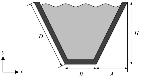
Trapezoidal cross section and flow channel.
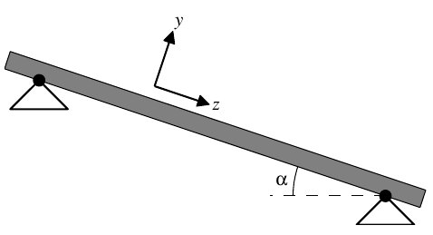
Given \(B\) and \(H\), the geometrical parameters \(A\) and \(D\) can be calculated from: \[\begin{aligned} D = \frac{1}{2}(L-B),\quad\text{and}\quad A = \sqrt{\frac{1}{4}(L-B)^2-H^2}. \end{aligned}\] We are interested in the flowrate \(Q\) defined as the integral of the velocity \(u\) (normal to the cross section) over the cross section \(\Phi\): \[\begin{aligned} Q=\int_\Phi u\,dx\,dy. \end{aligned}\] The channel is at a slope of angle \(\alpha\), as shown in Figure 1, and the horizontal components of the gravitational force creates the pressure gradient for the downward flow. The governing equations are the Navier-Stokes equations, \[\begin{aligned} \boldsymbol{u}\cdot \nabla \boldsymbol{u} + \nabla p=\boldsymbol{f} + \nu \nabla^2\boldsymbol{u}. \end{aligned}\]
With the assumption of fully developed flow, these can be reduced to Poisson’s equation for the velocity component \(u\) normal to the channel cross section, \[\begin{aligned} -\nabla^2u=\frac{g\sin\alpha}{\nu}. \end{aligned}\] Here, \(g\) is the gravitational constant, and \(\nu\) is the kinematic viscosity of the fluid. For simplicity, we assume that \[\begin{aligned} \frac{g\sin\alpha}{\nu}=1. \end{aligned}\]
Along the walls of the channel the velocity is zero, and on the free surface a zero-stress condition (\(\frac{\partial u}{\partial n}=0\)) is assumed.
We will solve Poisson’s equation using a finite difference procedure. Due to symmetry we only consider half the channel section, as shown in Figure 2. The following boundary conditions are applied on the original domain: \[\begin{cases} \frac{\partial u}{\partial n}=0, & \textrm{in $P_1P_4$ and $P_4P_3$} \\ u=0, & \textrm{in $P_1P_2$ and $P_2P_3$} \end{cases}\]
To solve the problem, we map the half domain \(\Omega\) to a rectangular domain \(\hat{\Omega}\) and then solve the equations numerically using the finite difference method on \(\hat{\Omega}\). We use a regular grid with \((n+1)\times (n+1)\) points in the computational domain, giving square cells of size \(\Delta \xi=\Delta \eta=1/n\).

Geometrical transformation from the physical space to the computational domain.
Introduce a mapping \(T\) to transform the original domain \(\Omega\) (with coordinates \(x,y\)) to the unit square \(\hat{\Omega}\) (with coordinates \(\xi,\eta\)). Derive the equations and the boundary conditions in the new domain.
In the transformed domain, write down second-order accurate finite-difference schemes for the discretization of all the derivative terms in the interior of the domain, as well as for the boundary points. You do not have to derive special schemes for the corner points, use the left boundary scheme at corner \(P_4'\), and \(u=0\) at the other three corners. Also show how to evaluate the integral in the approximate flowrate \(\hat{Q}\) numerically in the computational domain.
Write a Julia function with the calling syntax
Q, x, y, u = channelflow(L, B, H, n)that solves the problem for given values of \(L\), \(B\), and \(H\), and grid size \(n\). To debug your program, calculate the solution and \(\hat{Q}\) using a grid size \(n=20\), for \(L=3.0\), \(B=0.5\), and \(H=1.0\), and compare your results with the sample solution in Figure 3.

Sample solution, for L = 3.0, B = 0.5, H = 1.0, and n = 20. The plots show the grid (left) and contour lines of the solution (right).
Make convergence plots and calculate the convergence rates for the error in the output \(\hat{Q}\). Do the calculation for \(L=3.0\), \(H=1.0\), and \(B=0.0, 0.5, 1.0\) (3 convergence plots). Verify that you obtain approximately second-order convergence. Use the grid sizes \(n=10, 20, 40, 80, 160, 320\). Since we don’t know the exact solution, use the solution for \(n=320\) as a reference.
Consider the PDE \[\begin{aligned} u_t = \kappa u_{xx} - \gamma u, \end{aligned}\] which models a diffusion with decay provided \(\kappa>0\) and \(\gamma>0\). Consider methods of the form \[\begin{aligned} U_j^{n+1} =U_j^n+{\frac{k\kappa}{2h^2}} [U_{j-1}^n-2U_j^n +U_{j+1}^n +U_{j-1}^{n+1} - 2U_j^{n+1} + U_{j+1}^{n+1}] - k\gamma[(1-\theta)U_j^n + \theta U_j^{n+1}] \end{aligned}\] where \(\theta\) is a parameter. In particular, if \(\theta=1/2\) then the decay term is modeled with the same centered-in-time approach as the diffusion term and the method can be obtained by applying the Trapezoidal method to the MOL formulation of the PDE. If \(\theta=0\) then the decay term is handled explicitly. For more general reaction-diffusion equations it may be advantageous to handle the reaction terms explicitly since these terms are generally nonlinear, so making them implicit would require solving nonlinear systems in each time step (whereas handling the diffusion term implicitly only gives a linear system to solve in each time step).
- By computing the local truncation error, show that this method is \(\mathcal{O}(k^p+h^2)\) accurate, where \(p=2\) if \(\theta = 1/2\) and \(p=1\) otherwise.
(continued in PS2)
Code Submission: Your Julia file needs to define the
functions assemblePoisson and channelflow, and
any other supporting functions and variables.