UC Berkeley Math 228B, Spring 2024, Problem Set 3

1. Show that linear Transfinite Interpolation for a 2D domain with straight sides (that is, a quadrilateral) is equivalent to bilinear interpolation between its four corner points.

2. Consider the domain \(\Omega\) bounded by the four curves: \[\begin{aligned} x_\mathrm{left} &= 0 \\ x_\mathrm{right} &= 1 \\ y_\mathrm{bottom}(x) &= 64Ax^3(1 - x)^3 \\ y_\mathrm{top}(x) &= 1 + Ax^3(6x^2 - 15x + 10) \end{aligned}\] where \(A=0.4\). The goal is to find mappings of the form \((x,y)=\boldsymbol{R}(\xi,\eta)\) from the unit square to \(\Omega\) using Transfinite Interpolation (TFI).

   

   1. Create the mapping using TFI with linear Lagrange interpolation. Implement your function as a Julia function with the syntax

       xy = tfi_linear(ξη)

      Note that the input \(\xi\eta\) and the output xy are both vectors of length 2. Illustrate the mapping by plotting a structured grid of size \(40\times 40\) with the plot_mapped_grid function from the mesh utilities notebook on the course webpage.

   2. Create the mapping using TFI with cubic Hermite interpolation. Use the extra degrees of freedom to produce a mapping with boundary orthogonality. That is, find \((x,y) = \boldsymbol{R}(\xi,\eta)\) such that in addition to mapping the unit square to \(\Omega\), it also has the properties that $$

      \[\begin{aligned} \frac{\partial \boldsymbol{R}}{\partial \xi} &= T\boldsymbol{n}_\mathrm{leftright}\text{ at }\xi=0\text{ and }\xi=1 \\ \frac{\partial \boldsymbol{R}}{\partial \eta} &= T \boldsymbol{n}_\mathrm{bottom}(\xi)\text{ at }\eta=0\text{ and } \frac{\partial \boldsymbol{R}}{\partial \eta} = T \boldsymbol{n}_\mathrm{top}(\xi)\text{ at }\eta=1 \end{aligned}\]

      $$ where \(T\) is a parameter, \(\boldsymbol{n}_\mathrm{leftright}=[1,0]\) is the normal vector on the left and the right boundaries, and \(\boldsymbol{n}_\mathrm{bottom}(\xi),\boldsymbol{n}_\mathrm{top}(\xi)\) are the unit normal vectors on the bottom and the top boundaries, respectively (directed in the positive \(\eta\) direction). Implement the mapping in Julia as

            xy = tfi_orthogonal(ξη)

      and illustrate it by plotting a structured grid of size \(40\times 40\) with \(T=1/2\). Hint: While you could derive the full Hermite TFI form, for this particular problem it is sufficient to determine \(\boldsymbol{R}\) and its derivative \(\boldsymbol{R}_\eta\) on the bottom/top boundaries and only use Hermite interpolants in \(\eta\): \[\begin{aligned} \hat{\boldsymbol{R}}(\xi,\eta) = \Pi_\eta\boldsymbol{R} = \Big[ \boldsymbol{R}(\xi,0), \boldsymbol{R}(\xi,1), \boldsymbol{R}_\eta(\xi,0), \boldsymbol{R}_\eta(\xi,1) \Big] \cdot \Big[ H_0(\eta), H_1(\eta), \tilde{H}_0(\eta), \tilde{H}_1(\eta) \Big] \end{aligned}\]

3. Find the image of the rectangle \(0\le \mathrm{Re}(z)\le 1\), \(0\le \mathrm{Im}(z)\le 2\pi\) under the mapping \[\begin{aligned} w = \frac{2e^{z} - 3}{3e^{z} - 2} \end{aligned}\] and describe it in words or in mathematical notation (with full derivation, not just a plot). Use this to generate a structured grid of size \(20\times 80\) for this region with grid lines that are orthogonal everywhere.

4. Write a Julia function with the syntax

         p, t, e = pmesh(pv, hmax, nref)

   which generates an unstructured triangular mesh of the polygon with vertices pv, with edge lengths approximately equal to \(h_\mathrm{max}/2^{n_\mathrm{ref}}\), using a simplified Delaunay refinement algorithm. The outputs are the node points p (\(N\)-by-2), the triangle indices t (\(T\)-by-3), and the indices of the boundary points e.

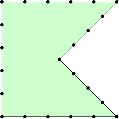
   1. The 2-column matrix pv contains the vertices \(x_i,y_i\) of the original polygon, with the last point equal to the first (a closed polygon).

   2. First, create node points along each polygon segment, such that all new segments have lengths \(\le h_\mathrm{max}\) (but as close to \(h_\mathrm{max}\) as possible). Make sure not to duplicate any nodes.

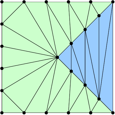
   3. Triangulate the domain using the delaunay function in the mesh utilities.

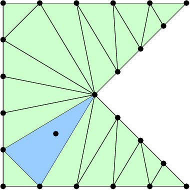
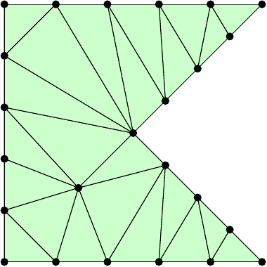
   4. Remove the triangles outside the domain (see the inpolygon command in the mesh utilities) as well as the almost degenerate triangles having an area less than \(\varepsilon=10^{-12}\).

   5. Find the triangle with largest area \(A\). If \(A>h_\mathrm{max}^2/2\), add the circumcenter of the triangle to the list of node points.

   6. Retriangulate and remove outside triangles (steps (c)-(d)).

   7. Repeat steps (e)-(f) until no triangle area \(A>h_\mathrm{max}^2/2\).

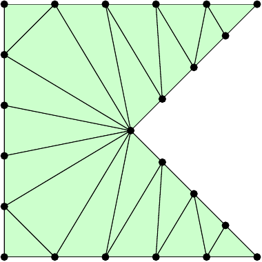
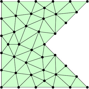
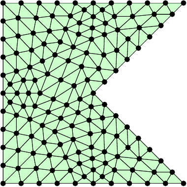
   8. Refine the mesh uniformly \(n_\mathrm{ref}\) times. In each refinement, add the center of each mesh edge (see all_edges) to the list of node points, and retriangulate.

   Finally, find the nodes e on the boundary using the boundary_nodes function. The following commands create the example in the figures. Also make sure that the function works with other inputs, that is, other polygons, \(h_\mathrm{max}\), and \(n_\mathrm{ref}\).

         pv = [0 0; 1 0; .5 .5; 1 1; 0 1; 0 0]
         p, t, e = pmesh(pv, 0.2, 1)
         tplot(p, t)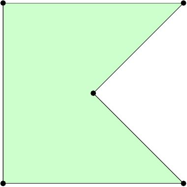

   
   
   
   
   
   
   
   

   
   

   
   
   
   
   
   
   
   

Code Submission: Your Julia file needs to define the functions tfi_linear, tfi_orthogonal, and pmesh, with exactly the requested names and input/output arguments, as well as any other supporting functions and variables that are required for your functions to run correctly.