UC Berkeley Math 228B, Spring 2024, Problem Set 5

In this problem set, you will study two extensions of the simple piece-wise linear Poisson solver fempoi from the previous problem set. First, you will extend the equations to solve the Helmholtz equation, for simulation of wave propagation in waveguides. Next, you will extend the Poisson solver to use quadratic elements instead of linear.

1. Consider the following 2-D Helmholtz problem, for a given wave number \(k\) with normalized propagation velocity, and so-called Sommerfeld radiation conditions at the in/out boundaries: \[\begin{aligned} -\nabla^2 u - k^2 u &= 0, & &\text{ in }\Omega, &&(1) \\ \boldsymbol{n} \cdot \nabla u &= 0, & &\text{ on }\Gamma_\mathrm{wall} &&(2)\\ \boldsymbol{n} \cdot \nabla u + iku &= 0, & &\text{ on }\Gamma_\mathrm{out} &&(3)\\ \boldsymbol{n} \cdot \nabla u + iku &= 2ik, & &\text{ on }\Gamma_\mathrm{in} &&(4) \end{aligned}\] Here, the domain boundary \(\Gamma = \partial \Omega\) is decomposed into the three parts \(\Gamma = \Gamma_\mathrm{wall} \cup \Gamma_\mathrm{out} \cup \Gamma_\mathrm{in}\). For a computed solution \(u\), we will also calculate its intensity at the output boundaries: \[\begin{aligned} H(u) = \int_{\Gamma_\mathrm{out}} |u|^2\,ds, &&(5) \end{aligned}\] where \(|\cdot|\) is the complex absolute value.

   1. Derive a Galerkin finite element formulation for (1)-(4), for an appropriate space \(V_h\) of continuous piece-wise linear functions.

   2. Show that the discretized system can be written in the form \(A\boldsymbol{u} = \boldsymbol{b}\), where \[\begin{aligned} A = K -k^2 M + i k (B_\mathrm{in} + B_\mathrm{out}) \quad \text{and} \quad \boldsymbol{b} = 2 i k \boldsymbol{b}_\mathrm{in} &&(6) \end{aligned}\] for real matrices \(K,M,B_\mathrm{in},B_\mathrm{out}\) and a vector \(\boldsymbol{b}_\mathrm{in}\), which do not depend on the wave number \(k\). Give explicit expressions for the matrix/vector entries, involving the basis functions \(\varphi_i(\boldsymbol{x})\) for the space \(V_h\).

   3. Show that the transmitted intensity (5) for a finite element solution \(\boldsymbol{u}\) can be calculated as \(H(\boldsymbol{u}) = \boldsymbol{u}^H B_\mathrm{out} \boldsymbol{u}\).

2. For the implementation, consider a model test problem with wave number \(k=6\) and a straight channel domain of dimensions \(5\times 1\): \[\begin{aligned} \Omega &= \{ 0\le x \le 5, 0\le y \le 1 \} &&(7) \\ \Gamma_\mathrm{in} &= \{x=0, 0\le y\le 1 \} &&(8)\\ \Gamma_\mathrm{out} &= \{x=5, 0\le y\le 1 \} &&(9)\\ \Gamma_\mathrm{wall} &= \{0\le x \le 5, y=0\text{ or }y=1 \} &&(10) \end{aligned}\]

   1. Show that an exact solution to the Helmholtz problem (1)-(4) for the domain (7)-(10) is given by \(u_\mathrm{exact}(x,y) = e^{-ikx}\).

   2. Write a function which for a given triangular mesh p, t identifies the boundary edges corresponding to the wall, the in, and the out boundaries, respectively:
      

         ein, eout, ewall = waveguide_edges(p, t)

      Use the function all_edges() in the Mesh utilities notebook on the course web page to find all mesh edges, then assume that the in-boundary consists of all vertical edges with \(x=0\), and that the out-boundary consist of all vertical edges with \(x=5\).

   3. Write a function that computes the matrices \(K,M,B_\mathrm{in},B_\mathrm{out}\) and the vector \(\boldsymbol{b}_\mathrm{in}\) for a given mesh:
      

         K, M, Bin, Bout, bin = femhelmholtz(p, t, ein, eout)

   4. Solve the discretized problem on the meshes generated by
      

          pv = [0 0; 5 0; 5 1; 0 1; 0 0]
          p, t, e = pmesh(pv, 0.3, nref)

      where nref ranges from \(1\) to \(4\). Compute max-norm errors using the exact solution \(u_\mathrm{exact}\), plot errors vs. mesh size in a log-log plot, and estimate the order of convergence.

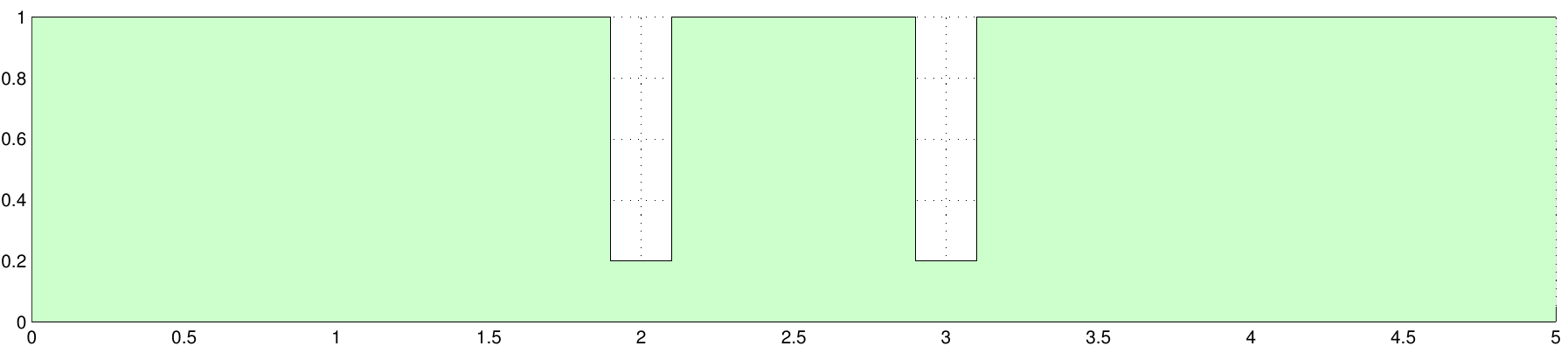
3. Finally, you will use your Helmholtz solver to compute a frequency response for a waveguide with two slits, see figure below. The waveguide is again of dimensions \(5\)-by-\(1\), and the slits are \(0.2\) units wide and \(0.8\) units deep, centered at \(x=2\) and \(x=3\).

   

   1. Create a mesh for the domain using pmesh, with hmax = 0.2 and nref = 2.

   2. To look for resonance phenomena around \(k\approx 2\pi\), solve for a range of wave numbers \(k\) between \(k=6\) and \(k=6.5\), in steps of \(\Delta k = 0.01\). For each \(k\), solve the problem and calculate \(H(\boldsymbol{u})\). Plot \(H\) vs. \(k\) in a semi-log plot.

   3. Plot two of your solutions using tplot of the real part, for the wave numbers \(k\) corresponding to the smallest and the largest value of \(H(\boldsymbol{u})\).

   Quadratic Elements for Poisson’s equation

4. Next you will modify the fempoi function to use quadratic elements instead of linear. Some details of the implementation:

   • Assume that all triangles are straight-sided

   • Use the following second-order accurate integration rule for a triangle \(T_k\) with corner nodes \(\boldsymbol{x}_1,\boldsymbol{x}_2,\boldsymbol{x}_3\) and area \(A_k\): \[\begin{aligned} \int_{T_k} f(\boldsymbol{x})\,d\boldsymbol{x} \approx A_k\sum_{i=1}^3 w^g_i f(\boldsymbol{x}^g_i),\ \ % w^g_i=1/3,\ \ \boldsymbol{x}^g_i = \sum_{j=1}^3 \left(\boldsymbol{x}_j/6 + \delta_{ij}\boldsymbol{x}_j/2 \right), \ \ i=1,2,3 \end{aligned}\]

   • Note that tplot only knows how to plot linear functions, but to plot a quadratic function you can at least use it to draw linear functions between the corner nodes:

        tplot(p, t, u[1:size(p,1)])

   1. First, a given mesh p,t has to be extended for quadratic functions by adding edge midpoints. Write a function
      

         p2, t2, e2 = p2mesh(p, t)

      which produces the arrays:

      p2

      : \(N\times 2\), node coordinates of original mesh nodes and the new midpoints

      t2

      : \(T\times 6\), local-to-global mapping for the \(T\) triangular elements

      e2

      : \(E\times 1\), indices of boundary nodes, both from original mesh nodes and the midpoints

      Use the function all_edges to find all mesh edges, and note the third output emap which is useful when creating t2.

   2. Write a function
      

         u = fempoi2(p2, t2, e2)

      which solves the Poisson problem using quadratic elements, for the mesh produced by your function p2mesh above.

   3. Do a convergence study as follows: Solve the problem on meshes given by
      

          hmax = 0.3
          pv = [0 0; 1 0; 1 1; 0 1; 0 0]
          p, t, e = pmesh(pv, hmax, nref)
          p2, t2, e2 = p2mesh(p, t)

      with homogeneous Dirichlet conditions on all boundaries and nref ranging from 0 to 4. Consider the finest mesh (nref = 4) the true solution. Calculate approximate max-norms for all the other solutions (nref = 0 to 3) as the maximum error at the set of nodes in the coarsest mesh (nref = 0). Plot these errors vs. mesh size in a log-log plot, and estimate the slope.

Code Submission: Your Julia file needs to define the functions waveguide_edges, femhelmholtz, p2mesh, fempoi2, with exactly the requested names and input/output arguments, as well as any other supporting functions and variables that are required for your functions to run correctly.