15.1. Graph Basics#
using Plots
15.1.1. What is a Graph?#
A graph is a way to represent relationships between objects. It consists of a set of vertices (or nodes) and a set of edges (or links) that connect pairs of vertices.
In a directed graph, edges have a direction (e.g., vertex A points to vertex B).
In an undirected graph, edges are bidirectional (e.g., A is connected to B).
15.1.1.1. Representing a Graph: Adjacency Lists#
There are many ways to represent a graph in a computer. A common and flexible method is an adjacency list.
We’ll number our vertices starting from \(1, 2, \ldots, n\).
We’ll have a main list (like an array) of all our vertices.
Each vertex object will then store its own list of neighbors, the indices of the other vertices it has an edge to.
To implement this, let’s first define a Julia struct to represent a single vertex. It will hold its list of neighbors and, for visualization, its 2D coordinates.
struct Vertex
    # A list of integers (indices) specifying which vertices this vertex points to
    neighbors::Vector{Int}

    # 2D coordinates [x, y] for plotting (optional)
    coordinates::Vector{Float64}

    # An inner constructor to provide a default value for coordinates
    Vertex(neighbors; coordinates=[0,0]) = new(neighbors, coordinates)
end

# This overloads the 'show' function to print a Vertex more nicely
function Base.show(io::IO, v::Vertex)
    print(io, "Neighbors = ", v.neighbors)
end
Now, the graph itself can be represented as a struct that simply contains a list (a Vector) of these Vertex objects. The index of a vertex in this list is its number (e.g., the vertex at g.vertices[3] is vertex 3).
struct Graph
    # A list containing all the Vertex objects in the graph
    vertices::Vector{Vertex}
end

# Overload 'show' to print the whole graph in a readable way
function Base.show(io::IO, g::Graph)
    for i = 1:length(g.vertices)
        println(io, "Vertex $i, ", g.vertices[i])
    end
end
15.1.1.2. Example: A Simple Directed Graph#
Let’s create a graph with 4 vertices. The connections will be:
  Vertex 1 -> Vertex 4
  Vertex 2 -> Vertices 1, 4
  Vertex 3 -> (No connections)
  Vertex 4 -> Vertex 2
We also provide \(x,y\) coordinates for plotting.
# Vertex 1 points to vertex 4
v1 = Vertex([4], coordinates=[1,0.5])

# Vertex 2 points to vertices 1 and 4
v2 = Vertex([1,4], coordinates=[0,2])

# Vertex 3 has no neighbors (an empty list)
v3 = Vertex([], coordinates=[-1,1])

# Vertex 4 points to vertex 2
v4 = Vertex([2], coordinates=[2,2])

# The graph is the collection of these vertices in order
g = Graph([v1,v2,v3,v4])
Vertex 1, Neighbors = [4]
Vertex 2, Neighbors = [1, 4]
Vertex 3, Neighbors = Int64[]
Vertex 4, Neighbors = [2]
15.1.2. Plotting a Graph#
The code below defines a custom plot recipe for our Graph struct. The result is that we can now just call plot(g) on a Graph object, and Plots.jl will know how to draw it using the coordinates and neighbor lists we provided.
You don’t need to understand the details of this function, just how to use it!
# This function tells Plots.jl how to handle an object of type 'Graph'
function Plots.plot(g::Graph; scale=1.0)
    # Get the bounding box of the coordinates to set plot limits
    xmin,xmax = extrema(v.coordinates[1] for v in g.vertices)
    ymin,ymax = extrema(v.coordinates[2] for v in g.vertices)

    sz = max(xmax-xmin, ymax-ymin)
    cr = scale*0.05sz # Circle radius
    hw = cr/2 # Not used here, but good for arrowheads

    # Set up a blank plot with no grid or axes, and equal aspect ratio
    plot(legend=false, grid=false, showaxis=false, aspect_ratio=:equal,
         xlims=[xmin-2cr, xmax+2cr], ylims=[ymin-2cr,ymax+2cr])

    # Points for drawing a circle
    npnts = 32
    ϕ = 2π*(0:npnts)/npnts
    cx,cy = cos.(ϕ), sin.(ϕ)

    # Draw each vertex as a circle with its number
    for i = 1:length(g.vertices)
        c = g.vertices[i].coordinates
        plot!(c[1] .+ cr*cx, c[2] .+ cr*cy, color=:black, linewidth=2)
        annotate!(c[1], c[2], text("$i", round(Int, 14*scale), :center))

        # For each neighbor, draw a directed edge (arrow)
        for nb in g.vertices[i].neighbors
            cnb = g.vertices[nb].coordinates
            dc = cnb .- c
            L = sqrt(sum(dc.^2))
            # Shorten the line so it starts/ends at the circle edge
            c1 = c .+ cr/L * dc
            c2 = cnb .- cr/L * dc
            plot!([c1[1],c2[1]], [c1[2],c2[2]],
                  arrow=:simple, color=:black, linewidth=2)
        end
    end
    return plot!() # Return the final plot
end

# Now we can just plot our graph object!
plot(g)

15.1.3. Creating Graphs Programmatically#
We can write functions to generate graphs. The function below creates an undirected cycle graph with nv vertices, arranged visually in a circle.
Note: to make an edge undirected, if vertex i points to vertex j, we must also make vertex j point to vertex i.
function circle_graph(nv=8)
    # Start with an empty graph
    g = Graph(Vertex[])

    for i = 1:nv
        # Calculate the angle for this vertex
        th = 2π*i/nv

        # Get neighbors: the vertex before (i-1) and after (i+1)
        # 'mod(i,nv)+1' is the next vertex, wrapping around from nv->1
        # 'mod(i-2,nv)+1' is the previous vertex, wrapping around from 1->nv
        neighbors = [mod(i,nv)+1, mod(i-2,nv)+1]

        # Create the vertex with its neighbors and coordinates
        v = Vertex(neighbors, coordinates=[cos(th), sin(th)])

        # Add the new vertex to the graph's list
        push!(g.vertices, v)
    end
    return g
end
circle_graph (generic function with 2 methods)
# Create and plot a 10-vertex circle graph
g = circle_graph(10)
plot(g)

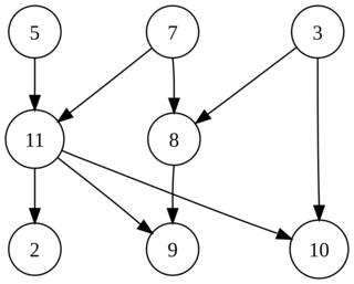
15.1.4. Modifying a Graph#
Because our graph is just a collection of Julia arrays, we can easily modify it using standard functions like push!, pop!, append!, and filter!.
# Start with a fresh 10-vertex circle graph
g = circle_graph(10)

# --- Add edges ---
# Add a single new edge from vertex 1 to 6
push!(g.vertices[1].neighbors, 6);
# Add two new edges from vertex 4 (to 2 and 7)
append!(g.vertices[4].neighbors, [2,7]);

# --- Change edges ---
# Change the first neighbor of vertex 3 to be vertex 1
g.vertices[3].neighbors[1] = 1

# --- Remove edges ---
# Remove the last neighbor from vertex 5's list
pop!(g.vertices[5].neighbors)

# --- Add a new vertex ---
# Note: The new vertex is #11 (the new length of g.vertices)
newv = Vertex([1,4,9], coordinates=[-.1,.3])
push!(g.vertices, newv)
# Add an edge from vertex 2 *to* our new vertex 11
push!(g.vertices[2].neighbors, 11)

# --- "Delete" a vertex (by removing all its edges) ---
# This is tricky, as it requires re-numbering all vertices.
# A simpler way is to just isolate it by removing its edges.
# Here, we isolate vertex 8.

# 1. Remove all *outgoing* edges from vertex 8
resize!(g.vertices[8].neighbors, 0)

# 2. Remove all *incoming* edges to vertex 8
for v in g.vertices
    # filter! keeps only neighbors 'i' that are NOT 8
    filter!(i -> i != 8, v.neighbors)
end

# Plot the final, modified graph
plot(g)
