17.2. Sparse Matrices in Julia

Julia supports sparse matrices in the SparseMatrixCSC type. It uses the CSC format, and the datatype Tv for the non-zeros and all indices Ti can optionally be specified, SparseMatrixCSC{Tv,Ti}.

Some special sparse matrices can be created using the following functions (together with their dense equivalents):

Sparse	Dense	Description
spzeros(m,n)	zeros(m,n)	m-by-n matrix of zeros
sparse(I, n, n)	Matrix(I,n,n)	n-by-n identity matrix
Array(S)	sparse(A)	Interconverts between dense and sparse formats
sprand(m,n,d)	rand(m,n)	m-by-n random matrix (uniform) of density d
sprandn(m,n,d)	randn(m,n)	m-by-n random matrix (normal) of density d

More general sparse matrices can be created with the syntax A = sparse(rows,cols,vals) which takes a vector rows of row indices, a vector cols of column indices, and a vector vals of stored values (essentially the COO format).

The inverse of this syntax is rows,cols,vals = findnz(A).

The number of non-zeros of a matrix A are returned by the nnz(A) function.

17.2.1. Example

For the matrix considered above, the easiest approach is to start from the COO format and use sparse(rows, cols, vals). The size of the matrix is determined from the indices, if needed it can also be specified as sparse(rows, cols, vals, m, n).

using PyPlot, SparseArrays, LinearAlgebra # Packages used

rows = [1,3,4,2,1,3,1,4,1,5]
cols = [1,1,1,2,3,3,4,4,5,5]
vals = [5,-2,-4,5,-3,-1,-2,-10,7,9]

A = sparse(rows, cols, vals, 5, 5)

5×5 SparseMatrixCSC{Int64, Int64} with 10 stored entries:
  5  ⋅  -3   -2  7
  ⋅  5   ⋅    ⋅  ⋅
 -2  ⋅  -1    ⋅  ⋅
 -4  ⋅   ⋅  -10  ⋅
  ⋅  ⋅   ⋅    ⋅  9

We note that Julia only displays the non-zeros in the matrix. If needed, it can be converted to a dense matrix:

Array(A)

5×5 Matrix{Int64}:
  5  0  -3   -2  7
  0  5   0    0  0
 -2  0  -1    0  0
 -4  0   0  -10  0
  0  0   0    0  9

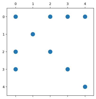
But in many cases, it is enough to only show the sparsity pattern of the matrix (not the actual values). PyPlot can visualize this using a so-called spy plot:

spy(A, marker=".", markersize=24);   ## Note - 0-based row and columns

17.2.2. Operations on sparse matrices

Many operations work exactly the same for sparse matrices as for dense matrices, including arithmetic operations, indexing, assignment, and concatenation:

B = A  - 4.3A   # Will automatically convert datatype of values to Float64
B[:,4] .= -1.1  # OK since B now has Float64 values (otherwise use Float64.(A) to convert)
C = A * A'      # Matrix multiplication (note: typically increases nnz)
Matrix([B C])   # Concatenation, again automatic conversion (of C)

5×10 Matrix{Float64}:
 -16.5    0.0  9.9  -1.1  -23.1  87.0   0.0  -7.0    0.0  63.0
   0.0  -16.5  0.0  -1.1    0.0   0.0  25.0   0.0    0.0   0.0
   6.6    0.0  3.3  -1.1    0.0  -7.0   0.0   5.0    8.0   0.0
  13.2    0.0  0.0  -1.1    0.0   0.0   0.0   8.0  116.0   0.0
   0.0    0.0  0.0  -1.1  -29.7  63.0   0.0   0.0    0.0  81.0

However, note that some standard operations can make the matrix more dense, and it might not make sense to use a sparse storage format for the result. Also, inserting new elements is expensive (for example the operation on the 4th column of B in the example above).

17.2.3. Incremental matrix construction

Since Julia uses the CSC format for sparse matrices, it is inefficient to create matrices incrementally (that is, to insert new non-zeros into the matrix). As an example, consider building a matrix using a for-loop. We start with an empty sparse matrix of given size \(N\)-by-\(N\), and insert a total of \(10N\) new random entries at random positions.

"""
Incremental matrix construction using the sparse-format
Not recommended: Insertion into existing matrix very slow
"""
function incremental_test_1(N)
    A = spzeros(N,N)
    for k = 1:10N
        i,j = rand(1:N, 2)
        A[i,j] = rand()
    end
    return A
end

incremental_test_1

We time the function for increasing values of \(N\):

incremental_test_1(10);   # Force compile before timing
for N in [100,1000,10000]
  @time incremental_test_1(N);
end

  0.000124 seconds (1.01 k allocations: 122.719 KiB)
  0.005774 seconds (10.02 k allocations: 1.409 MiB)
  0.771326 seconds (100.02 k allocations: 11.361 MiB)

We can observe the approximately quadratic dependency on \(N\), even though the number of non-zeros is only proportional to \(N\). This is because of the inefficiencies with element insertion into a sparse matrix.

Instead, we can build the same matrix using the COO format (row, column, and value indices) and only call sparse ones:

"""
Incremental matrix construction using COO and a single call to sparse
Fast approach, avoids incremental insertion into existing array
"""
function incremental_test_2(N)
    rows = Int64[]
    cols = Int64[]
    vals = Float64[]
    for i = 1:10N
        push!(rows, rand(1:N))
        push!(cols, rand(1:N))
        push!(vals, rand())
    end
    return sparse(rows, cols, vals, N, N)
end

incremental_test_2

incremental_test_2(10);   # Force compile before timing
for N in [100,1000,10000,100000,1000000]
  @time incremental_test_2(N);
end

  0.000042 seconds (28 allocations: 99.500 KiB)
  0.000494 seconds (41 allocations: 1.285 MiB)
  0.017001 seconds (50 allocations: 8.764 MiB, 55.91% gc time)
  0.115986 seconds (59 allocations: 62.151 MiB, 4.34% gc time)
  2.404683 seconds (71 allocations: 476.117 MiB, 0.28% gc time)

This version is magnitudes faster than the previous one, although it does not quite achieve linear dependency on \(N\) (possibly because of the sorting inside sparse).