12.3. The Convex Hull#
using Plots
default(legend=false, aspect_ratio=:equal)  # Set convenient defaults for all subsequent plots
12.3.1. Representing Points in Code#
In computational geometry, a fundamental building block is the point. For the 2D problems we’ll be exploring, a point is simply defined by its \((x,y)\) coordinates. In Julia, we can represent these coordinates as two Float64 numbers.
To store a collection of points, we have a few options. A common and efficient approach is to use a 2D array (a matrix) where each column represents a single point. For \(n\) points, this would be a 2 x n matrix. This structure is memory-efficient and makes certain operations very fast:
Accessing a single point (e.g., the i-th point):
p[:, i]Accessing all x- or y-coordinates:
p[1, :](all x-values) orp[2, :](all y-values)
The main trade-off is that adding a new point is less efficient, as it requires reallocating the array:
p = [p new_point] # This creates a new array
While packages like DynamicArrays.jl can optimize this, our current method is perfectly suitable for learning these algorithms.
# Generate a 2x10 matrix, representing 10 random points in a 2D plane.
p = randn(2, 10)
2×10 Matrix{Float64}:
  0.989617  -0.200196   0.98262  -0.904251  …   0.418002  0.800394  -1.06359
 -0.67067   -1.40891   -1.30156   1.46415      -0.491979  0.523615  -0.112504
# Create a scatter plot of the points.
# We use array slicing to pass all x-coordinates (the first row)
# and all y-coordinates (the second row) to the scatter function.
scatter(p[1,:], p[2,:])

12.3.2. The Convex Hull Problem#
The convex hull of a set of points \(X\) is the smallest convex set that contains all points in \(X\). Intuitively, imagine stretching a giant rubber band around all the points; the shape it forms is the convex hull.
Many algorithms exist to compute the convex hull. We will implement the Jarvis march, also known as the gift wrapping algorithm.
The algorithm proceeds as follows:
Start with the leftmost point \(p_0\) (the one with the minimum \(x\)-coordinate), which is guaranteed to be on the hull.
Find the next point \(p_1\) such that all other points lie to the right of the directed line from \(p_0\) to \(p_1\). This is like wrapping a rope tightly around the points.
Repeat this process, finding the next point in the sequence, until we arrive back at our starting point \(p_0\).
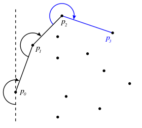
(Image from https://en.wikipedia.org/wiki/Gift_wrapping_algorithm)
12.3.2.1. Determining Point Orientation#
The core operation in the Jarvis march is determining if a point \(p_3\) is to the “left” or “right” of a directed line segment from \(p_1\) to \(p_2\). We can solve this using a clever trick from linear algebra: the cross product.
Consider two vectors: \(\vec{a} = p_2 - p_1\) and \(\vec{b} = p_3 - p_1\). The z-component of their cross product, \(\vec{a} \times \vec{b}\), tells us about their orientation:
If \(z > 0\), the turn from \(\vec{a}\) to \(\vec{b}\) is clockwise (i.e., \(p_3\) is to the right of the line \(p_1 \to p_2\)).
If \(z < 0\), the turn is counter-clockwise (i.e., \(p_3\) is to the left).
If \(z = 0\), the points \(p_1, p_2, p_3\) are collinear (all on the same line). For simplicity, our implementation won’t handle this special case.
function clockwise_oriented(p1, p2, p3)
    # Calculates the z-component of the cross product of the vectors (p2-p1) and (p3-p1).
    # Returns true if the orientation from vector p1->p2 to p1->p3 is clockwise.
    cross_product_z = (p2[1] - p1[1]) * (p3[2] - p1[2]) - (p2[2] - p1[2]) * (p3[1] - p1[1])

    # A positive result indicates a clockwise turn.
    return cross_product_z > 0
end
clockwise_oriented (generic function with 1 method)
# Test Cases
# Test 1: p3 = [2,3] is counter-clockwise ("left") of the vector from [0,0] to [1,1]. Should be false.
println(clockwise_oriented([0,0], [1,1], [2,3]))

# Test 2: p3 = [3,2] is clockwise ("right") of the vector from [0,0] to [1,1]. Should be true.
println(clockwise_oriented([0,0], [1,1], [3,2]))
true
false
With our orientation helper function, we can implement the full algorithm. Notice the nested loop structure:
An outer
whileloop adds one point to the hull at a time (\(p_0, p_1, \ldots\)). We use awhileloop because we don’t know in advance how many points will be on the hull.An inner
forloop iterates through all points in the set to find the next point on the hull. It finds the point that makes the most extreme clockwise turn relative to the current point.
This structure gives the algorithm a computational complexity of \(\mathcal{O}(nh)\), where \(n\) is the total number of points and \(h\) is the number of points on the convex hull.
function convex_hull(p)
    # Implements the Jarvis march (gift wrapping) algorithm to find the convex hull.

    # Step 1: Start with the leftmost point, which is guaranteed to be on the hull.
    # findmin returns the minimum value and its index; we only need the index.
    _, pointOnHull = findmin(p[1,:])

    # `hull` will store the indices of the points on the convex hull.
    hull = [pointOnHull]

    # Step 2 & 3: Repeatedly find the next point until we get back to the start.
    while length(hull) <= 1 || hull[1] != hull[end]
        # Pick an initial candidate for the next point. Any point other than the current one will do.
        # This modulo arithmetic is a simple way to wrap around and pick the 'next' point in the list.
        nextPoint = hull[end] % size(p, 2) + 1

        # Iterate through all points to find the one that makes the most clockwise turn.
        for j in 1:size(p, 2)
            # If point `j` is more clockwise than our current `nextPoint` candidate...
            if clockwise_oriented(p[:, hull[end]], p[:, nextPoint], p[:, j])
                # ...then we've found a better candidate.
                nextPoint = j
            end
        end
        # Add the best point found to our hull list.
        push!(hull, nextPoint)
    end

    return hull
end
convex_hull (generic function with 1 method)
# Example: Compute and draw the convex hull for 100 random points.
p = randn(2, 100)           # 1. Generate a new set of points.
hull = convex_hull(p)       # 2. Compute the hull, which returns a vector of indices.

scatter(p[1,:], p[2,:])     # 3. Plot all points as dots.
plot!(p[1,hull], p[2,hull]) # 4. Overlay the hull polygon by plotting the points at the hull indices.
