9.3. Linear Systems and Regression

using LinearAlgebra

9.3.1. Linear Systems

One of the most common uses of matrices is for solving linear systems of equations. Julia uses the backslash operator \ for this:

A = [1 2; 3 4]
b = [5,1]
x = A \ b         # Solve Ax = b for x

2-element Vector{Float64}:
 -9.0
  7.0

One way to view the syntax A\b is that it multiplies by A-inverse from the left, but using much more efficient and accurate algorithms.

To check that the answer is correct, we can use the \(\approx\) operator (since floating point numbers should never be compared exactly):

A*x ≈ b          # Confirm solution is correct

true

For systems with many right-hand side vectors b, the \ operator also works with matrices:

B = [5 7; 1 -3]
X = A \ B        # Solve for two RHS vectors

2×2 Matrix{Float64}:
 -9.0  -17.0
  7.0   12.0

 A*X ≈ B         # Confirm solution is correct

true

The algorithm used by the \ operator is typically Gaussian elimination, but the details are quite complex depending on the type of matrices involved. Due to the high cost of general Gaussian elimination, it can make a big difference if you use a specialized matrix type:

n = 2000
T = SymTridiagonal(2ones(n), -ones(n))     # n-by-n symmetric tridiagonal

for rep = 1:3 @time T \ randn(n) end       # Very fast since T is a SymTridiagonal
Tfull = Matrix(T)                          # Convert T to a full 2D array
for rep = 1:3 @time Tfull \ randn(n) end   # Now \ is magnitudes slower

  0.134713 seconds (389.64 k allocations: 23.538 MiB, 99.96% compilation time)
  0.000025 seconds (4 allocations: 63.000 KiB)
  0.000017 seconds (4 allocations: 63.000 KiB)
  0.216786 seconds (295.09 k allocations: 50.449 MiB, 3.38% gc time, 57.38% compilation time)
  0.104367 seconds (5 allocations: 30.564 MiB, 12.76% gc time)
  0.090345 seconds (5 allocations: 30.564 MiB)

The matrix A in A\b can also be rectangular, in which case a minimum-norm least squares solution is computed.

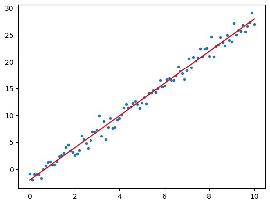
9.3.2. Linear regression

Suppose you want to approximate a set of \(n\) points \((x_i,y_i)\), \(i=1,\ldots,n\), by a straight line. The least squares approximation \(y=a + bx\) is given by the least-squares solution of the following over-determined system:

\[\begin{split} \begin{pmatrix} 1 & x_1 \\ 1 & x_2 \\ \vdots & \vdots \\ 1 & x_n \end{pmatrix} \begin{pmatrix} a \\ b \end{pmatrix}= \begin{pmatrix} y_1 \\ y_2 \\ \vdots \\ y_n \end{pmatrix} \end{split}\]

x = 0:0.1:10
n = length(x)
y = 3x .- 2 + randn(n)     # Example data: straight line with noise

A = [ones(n) x]            # LHS
ab = A \ y                 # Least-squares solution

using PyPlot
xplot = 0:10;
yplot = @. ab[1] + ab[2] * xplot
plot(x,y,".")
plot(xplot, yplot, "r");