6.2. Array Functions#
6.2.1. Introduction to Array functions#
We have seen before how many for-loops over arrays can be avoided using e.g. the dot-operator, which evaluates functions and operators element-wise. A number of other helper functions are available to extend this so-called vectorization technique, and allow for shorter code that is easier to understand and which might execute faster.
For example, a very common operation is to sum all the elements of an array. While this is easy to do with a for-loop, the function sum makes it even easier:
x = rand(1:100, 5)
println("Sum of ", x, " = ", sum(x))
Sum of [82, 12, 4, 59, 67] = 224
The sum function can also take an additional dimension argument dims, to specify which dimension it should add along. For example, it can add all the elements in each column (along dimension 1, producing a vector of sums):
A = rand(-100:100, 3, 5)
3×5 Matrix{Int64}:
 -35  -70  82   24  -33
  18    0  60   -4   65
   3   92  62  -60  -76
sum(A, dims=1)
1×5 Matrix{Int64}:
 -14  22  204  -40  -44
or it can add all the elements in each row (along dimension 2):
sum(A, dims=2)
3×1 Matrix{Int64}:
 -32
 139
  21
Note that while these functions reduce a 2D array to a 1D array, the output is still a 2D array (a row of a column vector). The syntax [:] after any array will convert it to a 1D array, which might be needed for example when using the array as indices.
sum(A, dims=1)[:]
5-element Vector{Int64}:
 -14
  22
 204
 -40
 -44
Some other examples of these so-called array reduction functions are shown below.
x = rand(1:100, 5)
display(x)
prod(x)                         # Product of all elements
5-element Vector{Int64}:
 31
 60
 62
 82
 85
803780400
display(A)
display(maximum(A, dims=1))     # Largest element in each column
display(minimum(A, dims=1))     # Smallest element in each column
3×5 Matrix{Int64}:
 -35  -70  82   24  -33
  18    0  60   -4   65
   3   92  62  -60  -76
1×5 Matrix{Int64}:
 18  92  82  24  65
1×5 Matrix{Int64}:
 -35  -70  60  -60  -76
The cumulative sum and product functions work in a similar way, but produce arrays of the same size as the original array:
x = 1:5
display(cumsum(x))                   # Cumulative sum, that is, entry n is the sum of x_1,...,x_n
display(cumprod(x))                  # Cumulative product
5-element Vector{Int64}:
  1
  3
  6
 10
 15
5-element Vector{Int64}:
   1
   2
   6
  24
 120
A = reshape(1:6, 2, 3)
2×3 reshape(::UnitRange{Int64}, 2, 3) with eltype Int64:
 1  3  5
 2  4  6
cumsum(A, dims=1) # Cumulative sum along dimension 1 (that is, column-wise)
2×3 Matrix{Int64}:
 1  3   5
 3  7  11
cumprod(A, dims=2) # Cumulative product along dimension 2
2×3 Matrix{Int64}:
 1  3  15
 2  8  48
6.2.2. Example: Taylor polynomial using array functions#
In part 1, we used for-loops to evaluate the Taylor polynomial for \(\cos x\) of a given degree \(2n\):
function taylor_cos(x,n)
    term = 1
    y = 1
    for k = 1:n
        term *= -x^2 / ((2k-1) * 2k)
        y += term
    end
    y
end
We can rewrite this in a vectorized form by using the cumprod and the sum functions. Note that each term in the sum is built up by multiplying the previous term by the expression -x^2 / ((2k-1) * 2k). This means we can create a vector with these values, and create all the terms using the cumprod function. Finally, the Taylor polynomial is obtained by adding all the terms using the sum function, and manually adding the first term 1 which is a special case:
function taylor_cos(x,n)
    factors = [ -x^2 / ((2k-1) * 2k) for k = 1:n ]
    y = 1 + sum(cumprod(factors))
end
taylor_cos (generic function with 1 method)
println(taylor_cos(10, 50)) # Taylor approximation
println(cos(10))            # true value
-0.8390715290752269
-0.8390715290764524
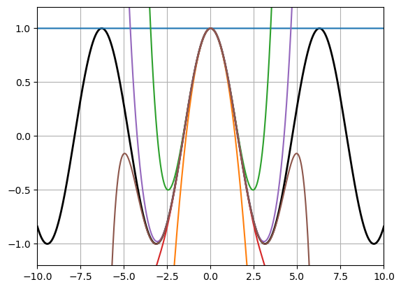
Since we now know how to plot functions, let us make the typical calculus plot that compares Taylor polynomial approximations of different degrees. Note how we can generate a 2D array yy_taylor of 6 different Taylor polynomials, for all values of x, using an array comprehension.
xx = -10:0.01:10
yy = cos.(xx)
yy_taylor = [ taylor_cos(x,n) for x in xx, n in 0:5 ]

using PyPlot
plot(xx, yy, linewidth=2, color="k")
plot(xx, yy_taylor)
grid(true)
axis([-10,10,-1.2,1.2]);
6.2.3. Array functions for indices and booleans#
Another useful set of array functions are based on indices and boolean variables. For example, the in function (or the \(\in\) symbol) will loop through an array and return true if a given number appears anywhere in the array:
x = 1:2:1000                 # Odd numbers
println(503 in x)            # True, 503 is in the list
println(1000 ∈ x)            # False, 1000 is not in the list
true
false
The all function returns true if all elements in a boolean array are true:
println(all(x .< 500))
println(all(x .> 0))
false
true
The any function returns true if any element in a boolean array is true:
println(any(x .== 503))
println(any(x .== 1000))
true
false
We can also find the index of e.g. the first element that is true in a boolean array:
idx = findfirst(x .== 503) # Index in x with the value 503
252
or more generally, a vector with the indices to all the elements that are true:
ind = findall(@. x % 97 == 0)
println("Indices in x with numbers that are multiples of 97: ", ind)
Indices in x with numbers that are multiples of 97: [49, 146, 243, 340, 437]
Finally, the count function returns the number of times true appears in a boolean array:
count(@. x % 97 == 0)
5